The Influence of Weight and Fat on Lamb Prices, Revisited
Charlie Hufton, Garry Griffith, John Mullen and Terence Farrell*
Charlie Hufton, lamb producer Harden and former BAgEc student, University of New England, Armidale.
Garry Griffith, Principal Research Scientist, NSW Department of Primary Industries, Armidale and Adjunct Professor, University of New England, Armidale.
John Mullen, Principal Research Scientist, NSW Department of Primary Industries, Orange, and Adjunct Professor, Charles Sturt University, Orange.
Terence Farrell, Consultant, Ag Economics, 11 Cynthia Crescent, Armidale.
Abstract
Previous research has found inconsistencies in the valuation of weight and fat characteristics of lamb carcasses between the saleyard and wholesale markets. In this paper, recent New South Wales saleyard, over-the-hook and wholesale price data on different classes of lamb are analysed using hedonic methods to determine the relative influence of weight and fat on prices received. In relation to fat score, lambs that are assessed as fat score 2 are discounted relative to lambs assessed as fat score 3, by around 26 c/kg in the live lamb market and by around 8 c/kg in the carcass market. There are no significant premiums or discounts for lambs assessed as fat score 4 in the markets where that could be tested. Premiums and discounts for fat scores are now consistent across the two market levels, and this implies some improvement in the efficiency of price discovery in the lamb market since Mullen’s study a decade ago. However, in relation to carcass weight, premiums and discounts are quite inconsistent across the market levels. There is a consistent premium for 18-20 kg lambs in all markets of between 11 and 40 c/kg, but then there is also a 29 c/kg premium for very light lambs in the wholesale market and a 38 c/kg premium for the heaviest lambs in the over-the-hook market. It appears that consumers’ stated preferences for larger lambs are not being reflected in price incentives generated in the live lamb and lamb carcass markets. Seasonal effects in all markets also proved to be significant, but the patterns are again quite different in each of the markets.
Keywords: lamb, marketing, hedonic models, carcass characteristics
1. Introduction
The Australian lamb industry has changed dramatically over the last decade or so[1]. Since 1995, the number of lambs slaughtered has risen 44 per cent and lamb carcass weight has risen 16 per cent, leading to a rise in the quantity of lamb produced of more than 60 per cent (ABARE 2008). Most of this extra output has been sold on export markets, exports having risen by two and half times the 1995 volume. This follows the introduction of the “large, lean lamb” program in the early 1990s (MRC 1992, Mullen and Alston 1994, Griffith et al. 1995). The range of export markets has expanded as have the types and qualities of lambs required. Australia is now one of the leading lamb producers in the world, and the second largest exporter of lamb. As well, there has been a concerted effort to improve the quality of lamb sold on the domestic market and a Meat Standards Australia scheme for sheep meat has been introduced.
Lamb prices received by producers are now driven by movements in export demands and exchange rates as well as by local pasture and seasonal conditions and economic and competitive conditions in the domestic meat market. While producers are unable to influence those factors determined in the rest of the economy, they can have some influence over the type of lamb produced. It is important then that price signals are efficiently transmitted through the lamb market so that there are appropriate incentives to produce those quality characteristics demanded by consumers in domestic and export markets. Understanding how lamb prices are determined, and what characteristics contribute to these prices, can be valuable to both buyers and producers. However, little research has been conducted on this issue in recent years. Mullen (1995) studied the influence of weight and fat score on the price of lamb in the Homebush livestock and wholesale markets, but that work used data that are now quite old. This study uses recent data to update the literature on this aspect of the Australian lamb market.
2. The Australian Lamb Industry
Australia is one of the world’s leading lamb producers, and the second largest exporter of lamb. In 2007 Australia produced 440 kt of lamb, with New South Wales and Victoria accounting for around two-thirds of this. In that year, the gross value of Australian lamb production was estimated at almost $1.5 billion. The number of lambs on hand at June 2007 was around 27 million, with the number of Merino and first cross lambs falling and the number of second cross lambs rising (MLA 2007).
Since the late 1980s, the lamb export market has become significantly more important to Australian lamb producers. In 1988, Australia exported only 16 per cent of lamb production, however 2007 saw Australian exports increase to around 45 per cent of total lamb production. Exports in 2007 were 192 kt, and the value of this lamb was estimated at $822 million (MLA 2007). Demand for Australian lamb has been stimulated by trade liberalisation in the United States, falling production in key lamb markets (particularly the United States and Europe), limited growth in exports from competitor countries like New Zealand, and rising demand in Asia as consumers look for alternative meats in the wake of disease outbreaks affecting beef and poultry (MLA 2007). The United States and North Asia are the principal trading regions for Australian lamb exports.
The domestic market, however, remains the most important sector of the lamb industry, taking some 55 per cent of all lamb produced. Most lamb (89 per cent) is sold through retail outlets, and 11 per cent is sold through the foodservice sector (MLA 2007). Despite a sharp decline in lamb demand in the 1980s and early 1990s, demand for lamb has recovered strongly since the late 1990s, despite being the meat with the largest price increases since 1998 (the lamb retail price index is over 70 per cent higher than prices in 1998) (see Figure 1). The average annual consumption per person in 2006/07 was 10.8 kgs (MLA 2007), with a total domestic utilisation of lamb of around 225 kt carcass weight. As a result, consumer expenditure on lamb has risen steadily over the years and is now estimated to be around $1.8 billion. Prices at the farm level have increased broadly in line with increases at the retail level.
Figure 1. Australian average lamb saleyard and retail prices, 1994-2006
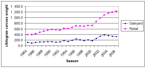
Source: ABARE (2008, Tables 154 and 155).
According to Meat and Livestock Australia (MLA), the increase in domestic demand has largely been in response to better quality lamb, a general rise in the healthy image of red meat, and successful marketing and promotion of lamb (MLA 2007). Consumers state that they prefer leaner and possibly larger lambs (Mullen and Wohlgenant 1991).
Producers may sell lambs in a number of ways (Table 1). The traditional method is the livestock saleyard. The saleyard system is based on averaging lambs of differing qualities in a pen on a dollar per head basis, which are then converted to c/kg estimated dressed weight by market reporters. Little objective feedback data is made available. The major saleyard markets are reported by the National Livestock Reporting Service (NLRS 2007), operated by MLA. During the 1997-1999 seasons approximately 87 per cent of prime lambs and 75 per cent of other lambs sold in New South Wales passed through the saleyard system. The percentage of lambs that passed through saleyards was lower in Victoria with 74 per cent of prime lambs and 70 per cent of other lambs. The remaining lambs were sold via paddock sales, over-the-hook or vertical alliance systems (Connell, Hooper and Brittle 2000).
Table 1. Method of lamb sales by State, 1998-1999
NSW |
NSW |
VIC |
VIC |
|
Prime |
Other |
Prime |
Other |
|
Lamb |
Lamb |
Lamb |
Lamb |
|
% |
% |
% |
% |
|
Auction sales |
86.8 |
75.2 |
74.2 |
69.7 |
Paddock sales |
9.8 |
7.2 |
13.0 |
20.4 |
Over the hook |
3.4 |
17.6 |
12.4 |
9.9 |
Other sales method |
0.0 |
0.0 |
0.3 |
0.0 |
Source: Connell, Hooper and Brittle (2000, Table 9, p. 30).
A growing sale method is over-the-hook (OTH), where producers sell directly to a processor and are then paid a c/kg price negotiated on the basis of actual carcass weight and fat score[2]. This method is beneficial to producers as they are paid for what they produce. Feedback is also readily available to producers regarding the details of the lambs sold. When producing so-called “elite lambs” that are both heavy and lean (22kg+, FS2/3 or leaner), this method of marketing can often be the most profitable.
Forward contracts are a marketing tool generally used by exporters who have made a commitment to overseas customers to supply them throughout the year. Forward contracts are legally binding agreements that are usually written two to six months prior to the agreed delivery date. The producer is paid on a c/kg basis, which is favorable for elite lambs that are finished to the target specifications.
The average weight of lambs has increased from 17 kgs in 1985 to 20.7 kgs in 2007 (ABARE 2008). Figure 2 shows the change in carcass weight during that period.
Figure 2. Average lamb carcass weight, 1985-2006
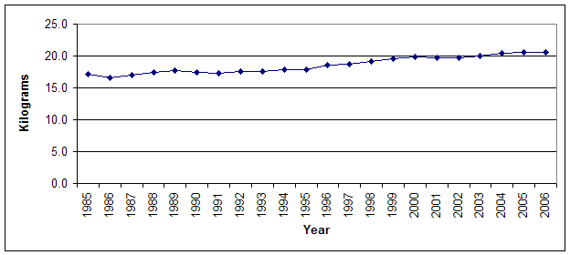
Source: ABARE (2008, Table 175).
The wholesale price for lamb in calculated for carcasses that pass through Sydney wholesale markets. Lamb production in New South Wales is bimodal with southern regions supplying the majority of lambs in late winter and spring, and northern markets supplying lambs in summer and autumn. For this reason it is expected that prices in southern New South Wales saleyards such as Wagga Wagga in late winter and spring should be highly correlated with Sydney wholesale prices during that period. In the alternate seasons, the wholesale market prices could be expected to correlate more with northern saleyard prices. Lambs purchased from the Wagga Wagga saleyards may be processed in Victoria and then the carcasses would be either sold in Victoria or returned to New South Wales or Queensland markets (Pers. Comm. Farrell, 2008).
Another consideration is that supermarkets such as Coles and Woolworths purchase a portion of their lamb supply direct from producers “on farm”. These two companies also source lambs direct from abattoirs and the value of this trade may not be recorded in the wholesale price series (Pers. Comm. Farrell, 2008).
3. Product Characteristics of Lamb
The value of lamb is driven by supply and it is contingent on weather in the short-term and the demand for wool and meat in the long-term. Retail yield was thought to be the most important driver of value for lamb carcasses. Retail yield is derived by subtracting the weight of fat trim and bone waste from the total weight of the carcass (Hopkins 1995). Considerable research has been focused on the valuation of carcasses at both the wholesale and retail levels. Thatcher and Couchman (1993), Hopkins, Wotton, Gamble and Atkinson (1995) and Hopkins, Fogarty and Farrell (1996) found that retailers preferred lambs that were between 17-18 kg and a maximum of 25 kg. The preferred fat score was 3 (15 mm GR). The discount for heavy lambs was reported to be $0.20/kg (Hopkins, Fogarty and Farrell 1996). During 1994-95, Hall, Farrell and MacDonald (1996) surveyed 44 retail butchers in Sydney and 59 per cent preferred lambs between 18-20 kg with fat score 2 and 38 per cent preferred lamb with fat score 3, one per cent preferred fat score 4. The discount for over fat lambs was reported as 21 per cent. The average preferred weight was 19 kg with 10 mm at the GR site. At that time only 9.2 per cent of the carcasses in three domestic abattoirs (Canberra, Cowra and Tamworth) they surveyed met those specifications.
More recently Farrell and Hopkins (2007) have shown that GR fat depth was poorly correlated with retail yield as the GR site measured both fat and lean muscle tissue depth at the 12th rib site. They also show that retailers and wholesalers value carcass conformation as being four times more important in price setting than either fat depth or retail yield. Carcass conformation can be measured on carcasses in abattoirs using Viascan technology; however, no mechanism is available to measure carcass confirmation on live animals. Sheep breed (genotype) has been used as a proxy for carcass conformation, however genotype was also poorly correlated with retailer and wholesaler valuations for different carcasses (Farrell and Hopkins 2007).
4. Previous Research
Mullen (1995) sought to establish the contribution of variation in fat cover and carcass weight to variations in the price of lamb in the Homebush livestock auction and wholesale markets. There were three main motivations for his analysis. Firstly, following Waugh’s (1928) argument that the contribution of quality factors to price variation ‘may prove to be fully as useful as the studies of factors causing the general level of price to change from day to day or from season to season’, Mullen believed that the producer has better control of the characteristics of a lamb therefore the study would benefit the producer in a way that would help them to understand what the market demands.
Secondly, he pointed out concerns in the lamb industry that there was a divergence between the values placed by consumers on fat cover and portion size, and the implicit prices received by producers for these quality factors in live lamb auction markets. Mullen (1995) asked the question whether efficiency gains in the lamb industry can be made by the development of a weight and grade selling system, where attributes such as weight and fat cover are explicitly valued and price divergence reduced.
The final motivation for Mullen’s study was to determine if there were different prices received for different characteristics in a lamb, and if there were, would it alter the buyer’s marginal implicit valuation of these characteristics.
He concluded, and confirmed widely held views, that price differentials for fat cover do exist in livestock auction and wholesale markets for lambs. Mullen reported that price premiums were paid for lambs with a fat score of 4 in the auction market and for a fat score of 3 in the wholesale market. In relation to premiums or discounts for the effect weight has on price, the results were less clearly represented, but there was a general consensus that premiums should be paid for heavier lambs because of savings in processing costs and because of attitudinal studies which suggested that consumers would prefer larger cuts of lamb (Mullen 1995). He further concluded that there was no strong evidence that in the livestock market, price differentials for fat score depended on the weight class and vice versa. Weight and fat interactions seemed to be more important in the wholesale market.
Mullen’s analysis clearly confirmed that buyers discriminate between lambs that differ in fat cover and weight. Additionally, he confirmed that the system of fat and weight classes used in the NLRS in both the livestock and wholesale markets, does indeed reflect differences in economic value to buyers in the markets. Mullen also noted the divergence observed in his study between price differentials for fat cover in the livestock and wholesale markets, and further that there was a divergence in the price differentials evident in these markets and perceived consumer preferences for leaner and perhaps larger lamb (Hopkins et al. 1985, Mullen and Wohlgenant 1991).
5. Model and Data
The current study has a similar range of motivations and related research questions. These research questions can be considered using hedonic models (see also Faminow and Gum 1986; Schroeder, Minert, Brazie and Grunewald 1988; Walburger 2002; Williams, Rolfe and Longworth 2003).
Hedonic Models
The basic idea of this type of analysis is to explain differences in prices received for various types of lamb (say between light ewe lambs and heavy wether lambs) by differences in their quality characteristics (such as fat cover, gender, age, etc). Two hedonic price specifications have been proposed in the literature to estimate these sorts of models (Mullen 1995). The first is the absolute price model:
- (1) Pi = aPr + S XijPj + ea
where Pi is the price of a particular class or type of lamb; Pr is the price of a reference type of lamb which has a given set of quality characteristics and which is selected to best reflect underlying supply and demand factors; Xij is the quantity of the characteristic j supplied by lamb type i; and Pj is the set of price differentials, away from the reference type, for a one unit change in the characteristic j. These differentials are coefficients estimated in the regression model and they can be positive (premiums, for a more-preferred characteristic) or negative (discounts, for a less-preferred characteristic). The underlying hypothesis of the absolute price model is that the estimated premiums and discounts for quality differences are constant - the differentials are independent of price levels. An error term is added for estimation.
The second specification is the relative price model:
- (2) Pi/Pr = b + S XijPj + er
where the variables are as defined above. The hypothesis here is that the quality differentials are proportional to price - as prices rise the differentials expand, and as prices fall the differentials contract.
These two specifications are tested against each other using non-nested tests reviewed by Doran (1993). Time series of sale data generated at a major saleyard, at over-the-hook sales and at the wholesale market were chosen to assess the research hypotheses.
Saleyard Data
A number of specific data choices have to be made to implement the various models:
* Selection of market. The NLRS report on a number of saleyard centres each week. Wagga Wagga saleyard was chosen as the representative market for this study. The NLRS report that for the year ending 30 June 2007, 1,951,000 sheep were sold through the Wagga Wagga yard, making it the largest selling centre in NSW. The next largest sale centre record is Forbes, with almost 500,000 less sheep sold than Wagga Wagga. During the years 2004/05, 2005/06 and 2006/07 (MLA 2007), Wagga Wagga has remained the number one selling centre for sheep, compared to any other centre in NSW.
Wagga Wagga has been quoted by market analysts and selling agents as being the best indicator lamb market for NSW. Lambs are drawn not only from the Riverina and Murrumbidgee areas, but also from the Upper Murray and South Eastern NSW. One of the main reasons for such a high percentage of lambs being sold in Wagga Wagga, is the ability of producers in the surrounding districts to supply lambs all year round. It is therefore widely accepted that the sales at Wagga Wagga will provide a greater variety of lambs in terms of composition and quality and, in turn, provide a better set of cross sectional data for evaluation.
* Selection of NLRS lamb quality characteristics. The NLRS reports contain a variety of information with the aim of providing accurate information regarding the market. Reports generally contain the following information:
- Fat score
- Category weight
- Sale percentage
- Dollars per head (low, high and average)
- Estimated carcass weight (low, high and average)
- Skin value (high and low)
From this list only two quality characteristics were chosen. These were carcass weight (4 possible classes – 16-18 kg, 18-20 kg, 20-22 kg and 22-24 kg) and fat score (3 possible classes - FS2, FS3 and FS4). Other factors known to influence price in particular markets such as age, breed, sex, grain finished and, finally, overall quality and condition, were excluded either because the variables are not reported by the NLRS or there were too few observations.
* Selection of lamb types. Based on the above choices, price data were collected for 12 different lamb types (4 weight classes and 3 fat score classes).
* Selection of reference type. One of these types has to be chosen as the reference type. Based on discussions with NLRS staff and producers and examination of sale numbers for each type, the reference type selected was 20-22 kg FS3 lambs. Thus the reference characteristics were 20-22 kg and FS3.
* Selection of time period. To obtain price series which covered different seasons and different market conditions, the time period selected was from 1 January 2006 to 30 December 2007. This resulted in a maximum number of 98 weekly sale observations for each of the lamb types. However, analysis of the sale data supplied by NLRS revealed that the three lighter weight ranges had very few if any FS4 reports, and that the heaviest weight range had very few FS2 reports. When these four classes were omitted (leaving 7 classes apart from the reference class), the maximum possible number of observations is therefore n=7*98=686. When all zero price observations in the remaining classes were deleted, n=499.
Final Saleyard Model
For each of the 7 non-reference lamb types, the price series for that type (Pi) and the reference price series (Pr) were entered as continuous series and the series for the quality characteristics were entered as dummy variables, where the dummy took the value zero if it was identical to the reference type and one if it was different. Thus there were five dummy variables for quality characteristics (D1618, D1820, D2224, DFS2, DFS4). The data set was then organised in panel format with the possible 98 observations on each of the 7 lamb types stacked vertically. Eleven monthly dummy variables were constructed and added to account for variations in pasture growth patterns, sheep breeding cycles and seasonality in demand for different types of meat, both domestically and in export markets. Where relevant, interactions between the quality characteristics were constructed and added, as were interactions between the seasonal variables and the characteristic interactions.
This resulted in final potential absolute and relative price models for the saleyard data of the general form[3]:
- (3) Pi = f (Pr, D1618, D1820, D2224, DFS2, DFS4, monthly seasonal dummies (11), characteristic interactions (6), seasonal interactions (55)), and
- (4) Pi/Pr = f (Constant, D1618, D1820, D2224, DFS2, DFS4, monthly seasonal dummies (11), characteristic interactions (6), seasonal interactions (55)).
It should be noted that in many cases, across each of the data sets, some of the characteristic interactions and/or seasonal interactions have to be omitted from the estimated models due to singularity problems.
Over-the-Hook Data
The NLRS also reports on producer over-the-hook sales direct to processors, with payment based on objective carcase measurements of weight and fat depth. In this market, lambs are traded by private treaty and hence the market report is based on the cooperation of processors in divulging prices that they pay for different types of lambs. The weekly reports include the following information:
- Weight Range
- Fat Score Range
- Average price
- Trend
As noted above, sales over-the-hook are growing in importance especially for larger lambs suitable for export contracts. With producers having an increasing range of options for selling their lambs, it is of interest to test whether the same types of signals for quality characteristics operate in both the saleyard and over-the-hook markets.
In organizing these data for analysis, the same procedures were followed as for the Wagga Wagga saleyard data. Five weight classes are available (the same as the saleyard classes plus a 24-26kg class) but the last category was excluded for consistency with the saleyard analysis. Unfortunately, only a consolidated fat score category of 2-4 is reported. The reference price chosen was therefore 20-22kg, FS2-4. Of the possible 4 weight classes over 98 weeks of data (294), 13 observations were removed for missing prices. This left n=281.
Final Over-the-hook Model
The final potential absolute and relative price models for the over-the-hook data are of the general form:
- (5) Pi = f (Pr, D1618, D1820, D2224, monthly seasonal dummies (11), characteristic interactions (0), seasonal interactions (33), and
- (6) Pi/Pr = f (Constant, D1618, D1820, D2224, monthly seasonal dummies (11), characteristic interactions (0), seasonal interactions (33).
Wholesale Data
The NLRS also reports on the wholesale market for lamb. The NLRS utilise the services of a trader from the Sydney wholesale market, who obtains data based on actual sales at the markets, together with information obtained from a number of other wholesalers. In the wholesale market, lambs are traded by private treaty and hence the market report is based on the cooperation of wholesalers in divulging prices that they receive for different types of lambs. The information collected from these sources is provided as a range and average. The NLRS takes this data and compiles it into a wholesale report which is published weekly. These reports generally consist of information including:
- Weight Range
- Fat Score
- Fat Depth
- Average price (lowest and highest prices)
- Trend
The same general procedures were followed. Here, there were 3 weight classes available (16-18 kg, 18-20 kg and 20+ kg) and 2 fat scores (FS2 and FS3). To align as closely as possible with the saleyard analysis, the reference price chosen was 20+kg, FS3. There were no FS2 lambs in the 20+kg weight range, and no missing data, so in total there are n=4*91=364 observations.
Final Wholesale Model
The final potential absolute and relative price models for the wholesale data are of the general form:
- (5) Pi = f (Pr, D1618, D1820, DFS2, monthly seasonal dummies (11), characteristic interactions (2), seasonal interactions (33), and
- (6) Pi/Pr = f (Constant, D1618, D1820, DFS2, monthly seasonal dummies (11), characteristic interactions (2), seasonal interactions (33).
Data Summary Statistics
The summary statistics for the final saleyard, over-the-hook and wholesale data sets are given in Table 2, 3 and 4 respectively. As expected, the saleyard reference price series (REF) has a higher mean and less variability than the Pi series (PRICE), since the latter contains a wider range of lamb types. The ratio variable used in the relative price model therefore has a mean less than one and quite high variability. This relationship is similar in the over-the-hook data, but the other way around in the wholesale data, although the means and standard deviations are very close in the latter data set. The means of the dummy variables generally reflect the expected proportions of those characteristics in the final data sets. There are slightly higher proportions of lighter lambs than heavier lambs in the saleyard data, and only 12 per cent have fat score 4, while in the over-the-hook data there are more heavier lambs than lighter lambs (as expected from the discussion in Section 2 above). In the wholesale data the proportions are exactly as expected. The reduced data sets do not appear to be biased across any of the quality measures.
Table 2: Saleyard data summary statistics
Number of Observations: 499 |
||||
Mean |
Std Dev |
Minimum |
Maximum |
|
PRICE |
321.70 |
50.29 |
88.00 |
413.00 |
REF |
329.15 |
36.72 |
218.80 |
387.00 |
PRATIO |
0.98 |
0.10 |
0.29 |
1.36 |
D1618 |
0.35 |
0.48 |
0.00 |
1.00 |
D1820 |
0.31 |
0.46 |
0.00 |
1.00 |
D2224 |
0.29 |
0.46 |
0.00 |
1.00 |
DFS2 |
0.34 |
0.47 |
0.00 |
1.00 |
DFS4 |
0.12 |
0.32 |
0.00 |
1.00 |
YARDING |
1646.00 |
1896.68 |
1.00 |
9259.00 |
Table 3: Over-the-hook data summary statistics
Number of Observations: 281 |
||||
Mean |
Std Dev |
Minimum |
Maximum |
|
PRICE |
314.31 |
40.21 |
210.00 |
378.00 |
REF |
328.29 3 |
30.49 |
252.00 |
376.00 |
PRATIO |
0.96 |
0.08 |
0.69 |
1.05 |
D1618 |
0.30 |
0.46 |
0.00 |
1.00 |
D1820 |
0.35 |
0.48 |
0.00 |
1.00 |
D2224 |
0.35 |
0.48 |
0.00 |
1.00 |
Table 4: Wholesale data summary statistics
Number of Observations: 364 |
||||
Mean |
Std Dev |
Minimum |
Maximum |
|
PRICE |
410.58 |
28.71 |
325.00 |
460.00 |
REF |
411.32 |
28.53 |
330.00 |
445.00 |
PRATIO |
0.99 |
0.02 |
0.94 |
1.07 |
D1618 |
0.50 |
0.50 |
0.00 |
1.00 |
D1820 |
0.50 |
0.50 |
0.00 |
1.00 |
DFS2 |
0.50 |
0.50 |
0.00 |
1.00 |
Figure 3 shows the relationship between the saleyard reference price and the other saleyard prices over all the 98 weekly observations, so there are many gaps in some prices. The whole array of prices generally moves together in a broad seasonal pattern, but there is considerable short term variability in all prices. It is particularly evident that the lighter, leaner lambs are sold down late in the year relative to their heavier peers.
Figure 3. The reference price (20-22kg, FS3) and other saleyard prices at Wagga Wagga, 2006-2007
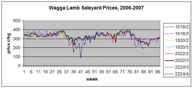
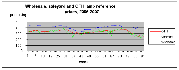
Figure 4 shows the relationship between the saleyard, over-the-hook and wholesale reference prices over all the 98 weekly observations. Again, the three prices generally move together in a broad seasonal pattern, but the considerable short term variability in the saleyard price is not reflected in either the over-the-hook or wholesale prices (as also indicated in the standard deviation values in the above tables).
Figure 4. Wagga saleyard, over-the-hook and wholesale lamb reference prices, 2006-2007
6. Estimation Results
Wagga Wagga Saleyard Market
The base absolute price model for the Wagga Wagga saleyard data is presented in Table 5. It shows the relationship between the reference price, which is for a lamb of 20 to 22 kgs with a fat score of 3, the price of all other categories of lamb, and the following dummy variables: D1618 (lamb weighing 16 to 18 kgs); D1820 (lamb weighing 18 to 20 kgs); D2224 (lamb weighing 22 to 24 kg); DFS2 (lamb with fat score 2) and DFS4 (lamb with fat score 4).
Table 5. Base absolute price saleyard model
Variable |
Estimated coefficient |
Standard error |
t-statistic |
P-value |
REF |
1.018 |
0.0171 |
59.46 |
[.000] |
D1618 |
-7.683 |
5.598 |
-1.37 |
[.171] |
D1820 |
-1.018 |
5.692 |
-0.179 |
[.858] |
D2224 |
-6.553 |
6.316 |
-1.037 |
[.300] |
DFS2 |
-27.976 |
3.043 |
-9.195 |
[.000] |
DFS4 |
9.292 |
4.709 |
1.973 |
[.049] |
Adjusted R-squared = 0.69; Mean of dep. var. = 321.7; Durbin-Watson = 1.48 [<.000]; Ramsey's RESET2 = 2.43 [.119]
Sixty nine per cent of variation was explained by the chosen variables. This relatively low level of explanation was to be expected given all the other possible influences on price differentials in the live animal market (age, breed, sex, grain finished and overall quality and condition) that are not accounted for by the specified independent variables. Positive autocorrelation existed within the estimated equation (and in most of the estimated equations) as evidenced by the Durbin-Watson statistic, however this statistic is not really relevant for this type of sequenced data. The RESET test suggests a well specified base model.
Not all the quality characteristics were significant. The weight dummy variables were not significant and this means that if the weight class was to change from that of the reference class, there would be no significant difference from the reference price. The coefficient for the FS2 variable was very significant and suggests a significant discount of around 28 c/kg for a FS2 lamb relative to a FS3 lamb. In this case there was also a significant premium of around 9 c/kg for FS4 lambs.
The model presented in Table 6 improved on the base absolute price model. Individually all but three of the seasonal variables had very significant coefficients and the F and Chi-squared tests showed they should be included as a group in the set of explanatory variables. The difference between the reference price and the other price series was higher in summer, autumn and early winter by between 17 and 27 c/kg. The 18-20 kg lambs were traded at a significant premium of 11 c/kg over 20-22 kg lambs, but no other variables showed any significant difference from zero. Again the FS2 variable was significant, showing that a discount of 26 c/kg would apply to a FS2 lamb in comparison to a FS3 lamb, and the premium for FS4 was around 7 c/kg now not significant. Overall the R-squared has improved a little but there were now signs of misspecification in the model.
Table 6. Absolute price saleyard model with seasonal effects
Variable |
Estimated coefficient |
Standard error |
t-statistic |
p-value |
REF |
.938 |
.023 |
39.79 |
[.000] |
D1618 |
4.961 |
5.577 |
.89 |
[.374] |
D1820 |
11.289 |
5.678 |
1.99 |
[.047] |
D2224 |
7.874 |
6.288 |
1.25 |
[.211] |
DFS2 |
-25.918 |
2.863 |
-9.05 |
[.000] |
DFS4 |
7.012 |
4.375 |
1.60 |
[.110] |
JAN |
21.919 |
7.079 |
3.10 |
[.002] |
FEB |
27.454 |
7.075 |
3.88 |
[.000] |
MAR |
21.172 |
.780 |
3.12 |
[.002] |
APR |
21.150 |
7.908 |
2.67 |
[.008] |
MAY |
27.600 |
7.077 |
3.90 |
[.000] |
JUN |
17.105 |
7.226 |
2.37 |
[.018] |
JUL |
17.604 |
7.448 |
2.36 |
[.018] |
AUG |
-1.740 |
6.665 |
-.26 |
[.794] |
SEP |
1.265 |
6.339 |
.20 |
[.842] |
OCT |
-12.163 |
6.258 |
-1.94 |
[.053] |
NOV |
8.203 |
6.783 |
1.21 |
[.227] |
Adjusted R-squared = 0.74; Mean of dep. var. = 321.7; Durbin-Watson = 1.70 [<.009];Ramsey's RESET2 = 25.2 [.000]; F(11,493) Test Statistic: 8.87, Upper tail area: .00000CHISQ(11) Test Statistic: 90.16, Upper tail area: .00000
Several other absolute price models were estimated that included the fat score/weight interaction variables and the seasonal/fat score and seasonal/weight interaction variables as mentioned above, but none of the groups of interaction terms proved to be significant on the basis of the calculated F and LLR tests and were therefore discarded. Two individual interaction terms were significant at the 10 per cent level, confirming that discounts for FS2 lambs were greater at lower weights. Specification tests for functional form were also run, but these were inconclusive. The linear model as reported above was retained for ease of interpretation.
The relative price saleyard model was estimated using the same procedures as for the absolute price model. In the preferred model, some 29 per cent of the variation in the price ratio is explained by the estimated model (Table 7). This much lower level of explanatory power is to be expected given the highly variable nature of the dependent variable. The seasonal dummy variables are highly significant as a group and many are significant individually. The FS2 dummy variable again suggests a significant discount for FS2 lambs relative to FS3 lambs (calculated to be 25 c/kg at the price means), but there are no other significant quality effects.
Table 7. Relative price saleyard model with seasonal effects
Variable |
Estimated coefficient |
Standard error |
t-statistic |
P-value |
C |
.973 |
.029 |
33.70 |
[.000] |
D1618 |
.001 |
.020 |
.03 |
[.974] |
D1820 |
.022 |
.021 |
1.08 |
[.283] |
D2224 |
.013 |
.023 |
.58 |
[.559] |
DFS2 |
-.087 |
.010 |
-8.78 |
[.000] |
DFS4 |
.019 |
.015 |
1.25 |
[.213] |
JAN |
.046 |
.024 |
1.93 |
[.055] |
FEB |
.061 |
.023 |
2.61 |
[.009] |
MAR |
.043 |
.023 |
1.90 |
[.058] |
APR |
.045 |
.027 |
1.65 |
[.100] |
MAY |
.069 |
.024 |
2.94 |
[.003] |
JUN |
.028 |
.023 |
1.21 |
[.227] |
JUL |
.027 |
.023 |
1.14 |
[.256] |
AUG |
-.027 |
.023 |
-1.16 |
[.246] |
SEP |
-.017 |
.024 |
-.71 |
[.479] |
OCT |
-.058 |
.024 |
-2.43 |
[.015] |
NOV |
.007 |
.025 |
.30 |
[.766] |
As with the absolute price model, none of the groups of interaction terms proved to be significant on the basis of the calculated F and LLR tests, and the specification tests for functional form were again inconclusive.
Finally the absolute and relative price models were tested against each other using J and JA tests. Two of the four test statistics rejected the relative price model and the other two rejected the absolute price model, so neither dominates. This is not seen as a problem as both models estimate approximately the same discount for FS2 lambs.
Over-the Hook Market
The over-the-hook market models are similar to those of the livestock auction market, except that the number of quality variables is much less (just weight categories). The same general procedure was followed with respect to the addition of seasonal and interaction terms, the testing of functional form, and the comparison of the absolute and relative price models.
The preferred absolute price over-the-hook model with seasonal effects included is shown in Table 8.
Table 8. Absolute price over-the-hook model with seasonal effects
Variable |
Estimated coefficient |
Standard error |
t-statistic |
P-value |
REF |
.851 |
.057 |
14.83 |
[.000] |
D1618 |
-7.196 |
18.094 |
-.40 |
[.691] |
D1820 |
40.780 |
18.094 |
2.25 |
[.025] |
D2224 |
38.485 |
18.094 |
2.13 |
[.034] |
JAN |
8.220 |
5.234 |
1.57 |
[.118] |
FEB |
10.444 |
5.415 |
1.93 |
[.055] |
MAR |
4.599 |
5.455 |
.84 |
[.400] |
APR |
6.367 |
5.325 |
1.20 |
[.233] |
MAY |
12.893 |
5.508 |
2.34 |
[.020] |
JUN |
20.699 |
5.158 |
3.36 |
[.001] |
JUL |
18.814 |
5.975 |
3.15 |
[.002] |
AUG |
13.778 |
5.304 |
2.60 |
[.010] |
SEP |
7.964 |
5.149 |
1.55 |
[.123] |
OCT |
5.498 |
5.024 |
1.09 |
[.275] |
NOV |
3.659 |
5.075 |
.72 |
[.472] |
Here, 87 per cent of the variation in the price variable can be explained by the chosen variables, which is a substantial improvement over the equivalent saleyard model. The over-the-hook market is essentially a carcase market, and different carcasses have different end uses depending on weight and fat score and the other factors that influence saleyard price are less important. There is evidence of substantial positive autocorrelation but the RESET test suggests a well specified model.
The significance of the quality characteristics is very different to those of the saleyard model. The 18-20 kg and 22-24 kg weight dummy variables are significant and this means that if the weight class was to change from that of the reference class, there would be a significant premium from doing so of around 40 c/kg. However there could be some confounding with fat score in these results as the prices for these weight classes are given for a fat score range of 2-4.
Individually the monthly variables for May through to August have very significant coefficients suggesting premiums during these months, and the F and Chi-squared tests show that all seasonal variables should be grouped by seasons. By selling in late autumn and winter, the vendor will receive a price premium of between 13 and 20 c/kg. It is interesting to note that unlike the livestock market, where a premium was received for lambs sold in early autumn, this is not the case in the over-the-hook market.
Including the full set of quality/seasonal interactions did result in significant F and Chi-squared test statistics, but no individual interaction terms were significant and there was little change in the size or significance of any of the other coefficients, so the groups of interactions were omitted from the preferred model. Specification tests for functional form were inconclusive (two tests rejected the log form and one test rejected the linear form) so the linear model was retained.
The relative price over-the-hook model was estimated using the same procedures as for the absolute price model. The results are shown in Table 9.
Table 9. Relative price over-the-hook model with seasonal effects
Variable |
Estimated coefficient |
Standard error |
t-statistic |
P-value |
C |
.833 |
.014 |
60.81 |
[.000] |
D1820 |
.149 |
.007 |
22.06 |
[.000] |
D2224 |
.142 |
.007 |
21.05 |
[.000] |
JAN |
.018 |
.016 |
1.10 |
[.274] |
FEB |
.022 |
.016 |
1.35 |
[.178] |
MAR |
.004 |
.016 |
.27 |
[.788] |
APR |
.010 |
.016 |
.64 |
[.521] |
MAY |
.026 |
.016 |
1.66 |
[.099] |
JUN |
.042 |
.017 |
2.51 |
[.013] |
JUL |
.037 |
.016 |
2.29 |
[.023] |
AUG |
.035 |
.016 |
2.12 |
[.035] |
SEP |
.032 |
.016 |
2.01 |
[.045] |
OCT |
.025 |
.016 |
1.63 |
[.104] |
NOV |
.016 |
.016 |
1.00 |
[.318] |
Some 69 per cent of the variation in the price ratio is explained by the estimated model, which again is quite an improvement over the equivalent saleyard model. The summary statistics suggest misspecification. The seasonal dummy variables are highly significant as a group, and individually during the winter and early spring period. In contrast to the saleyard results, there is a significant premium for lambs that are both lighter and heavier than the reference class.
None of the groups of interaction terms proved to be significant on the basis of the calculated F and LLR tests, and the specification tests for functional form were again inconclusive, so the linear model was retained for ease of interpretation.
Finally the absolute and relative price models were tested against each other using J and JA tests. All four test statistics rejected the null hypothesis, so the results relating to the preferred functional form are again inconclusive.
Sydney Wholesale Market
The same general procedure was followed with respect to estimation and testing of the wholesale market models. The absolute price wholesale model with seasonal effects included is shown in Table 6.
Table 10. Absolute price wholesale model with seasonal effects
Variable |
Estimated coefficient |
Standard error |
t-statistic |
P-value |
REF |
.916 |
.015 |
59.41 |
[.000] |
D1618 |
28.852 |
5.995 |
4.81 |
[.000] |
D1820 |
34.951 |
5.995 |
5.83 |
[.000] |
DFS2 |
-7.527 |
.661 |
-11.39 |
[.000] |
JAN |
16.780 |
2.272 |
7.39 |
[.000] |
FEB |
12.407 |
2.009 |
6.18 |
[.000] |
MAR |
2.548 |
2.006 |
6.25 |
[.000] |
APR |
12.587 |
2.072 |
6.08 |
[.000] |
MAY |
9.329 |
2.037 |
4.58 |
[.000] |
JUN |
.985 |
2.153 |
.46 |
[.648] |
JUL |
1.582 |
2.116 |
.75 |
[.455] |
AUG |
1.579 |
2.052 |
.77 |
[.442] |
SEP |
.740 |
2.050 |
.36 |
[.718] |
OCT |
.526 |
1.949 |
.27 |
[.787] |
NOV |
-.289 |
1.894 |
.15 |
[.879] |
Here, 95 per cent of the variation in the price variable can be explained by the chosen variables, which is a substantial improvement over the equivalent saleyard and over-the-hook models. At the wholesale level there is further differentiation based on end uses and the other factors that influence price are less important.
All quality characteristics are significant. The two weight dummy variables are significant and this means that if the weight class was to decrease from that of the reference class, there would be a significant premium from doing so of up to 35 c/kg. The coefficient for the FS2 variable is significant with a high t-statistic, suggesting a discount of around 7 c/kg for a FS2 lamb relative to a FS3 lamb.
Individually the monthly variables for January through to May have very significant coefficients suggesting premiums during these months, and the F and Chi-squared tests show that all seasonal variables should be included as a group. By selling in late summer and autumn, the vendor will receive a price premium of between 9 and 16 c/kg. This is more like the saleyard seasonal pattern than that in the over-the-hook market.
The full set of quality/seasonal interactions were omitted from the preferred model based on the F and Chi-squared tests, and specification tests for functional form were inconclusive so the linear model was retained.
The relative price wholesale model was estimated using the same procedures as for the absolute price model.
Table 11. Relative price wholesale model with seasonal effects
Variable |
Estimated coefficient |
Standard error |
t-statistic |
p-value |
C |
1.009 |
.004 |
243.47 |
[.000] |
D1618 |
-.015 |
.002 |
-9.06 |
[.000] |
DFS2 |
-.018 |
.002 |
-11.02 |
[.000] |
JAN |
.036 |
.006 |
6.36 |
[.000] |
FEB |
.024 |
.005 |
4.94 |
[.000] |
MAR |
.023 |
.005 |
4.72 |
[.000] |
APR |
.023 |
.005 |
4.60 |
[.000] |
MAY |
.012 |
.005 |
2.56 |
[.011] |
JUN |
-.008 |
.005 |
-1.58 |
[.116] |
JUL |
-.007 |
.005 |
-1.52 |
[.129] |
AUG |
-.006 |
.005 |
-1.24 |
[.217] |
SEP |
-.005 |
.005 |
-1.02 |
[.308] |
OCT |
-.002 |
.005 |
-.49 |
[.622] |
NOV |
-.002 |
.005 |
-.32 |
[.753] |
As shown in Table 11, some 56 per cent of the variation in the price ratio is explained by the estimated model. The seasonal dummy variables are highly significant as a group and follow the same pattern as in the absolute price model. The FS2 dummy variable again suggests a significant discount for FS2 lambs relative to FS3 lambs (around 7 c/kg), and in this model there is a significant discount for 16-18kg lambs relative to 20+kg lambs.
None of the groups of interaction terms proved to be significant on the basis of the calculated F and LLR tests, and the specification tests for functional form were again inconclusive.
Finally the absolute and relative price models were tested against each other using J and JA tests. All four test statistics either rejected the relative price model or could not reject the absolute price model. This suggests that for the wholesale data at least, the absolute price model provides the better explanation of premiums and discounts in wholesale lamb prices due to carcass quality attributes.
7. Summary and Conclusion
The linear versions of the absolute price models (Tables 6, 8 and 10) appear to best explain price behaviour in relation to quality characteristics in the New South Wales lamb market. The key results are summarized in Table 12.
Table 12. Comparison of the absolute price saleyard, over-the-hook and wholesale models, with seasonal effects
Variable |
Saleyard Coefficient (p-value) |
Over-the-hook Coefficient (p-value) |
Wholesale Coefficient (p_value) |
REF |
0.938 [.000] |
0.851 [.000] |
0.961 [.000] |
D1618 |
4.961 [.374] |
-7.196 [.691] |
28.852 [.000] |
D1820 |
11.289 [.047] |
40.780 [.025] |
34.951 [.000] |
D2224 |
7.874 [.211] |
38.485 [.034] |
|
DFS2 |
-25.918[.000] |
-7.527 [.000] |
|
DFS4 |
7.012 [.110] |
||
Significant seasonal effects |
Jan-Jul, Oct |
Feb,May-Aug |
Jan-May |
The results certainly indicate that different values do apply for different quality characteristics in the lamb and carcass markets analysed. In relation to fat score, lambs that are assessed as fat score 2 are discounted relative to fat score 3 lambs, by around 26 c/kg in the live lamb market and by around 8 c/kg in the carcass market. There are no significant premiums or discounts for fat score 4 lambs relative to fat score 3 lambs in the markets where that could be tested. Premiums and discounts for fat scores are now consistent across the two market levels, and this implies some improvement in the efficiency of price discovery in the lamb market since Mullen’s study a decade ago. However there is still a divergence between consumers’ stated preferences for leaner lambs (Hopkins et. al 1985, Mullen and Wohlgenant 1991) and the price incentives generated in the live lamb and lamb carcass markets. This is backed up by the positive though not significant premium for fat score 4 lambs relative to fat score 3 lambs in the saleyard market. Further, there is a marked difference in the discount applying to FS2 lambs at the saleyard and wholesale levels. This no doubt reflects the difference sources of risk in the two markets, where in the saleyard buyers have to estimate wool length and type as well as fat score in the live animal.
In relation to carcass weight, premiums and discounts due to differences in weight in lambs and in carcasses are inconsistent across the market levels. There is a consistent premium for 18-20 kg lambs relative to 20-22 kg lambs in all markets of between 11 and 40 c/kg, but then there is also a 29 c/kg premium for very light lambs in the wholesale market and a 38 c/kg premium for the heaviest lambs in the over-the-hook market. This finding is perhaps due to the expansion in the range of market outlets available for lamb, and the specialization of different markets for lambs of different sizes.
Seasonal effects in all markets proved to be significant, but the patterns are also quite different in each of the markets. In the livestock auction market, premiums are paid for lambs that are sold in summer, autumn and winter compared to those sold in spring. A producer is able to receive at least 17 c/kg more by selling lambs in early in the year as opposed to later in the year. The over-the-hook market shows a more variable seasonal pattern but premiums of up to 20 c/kg are available for sales in May through to August. Seasonal variables in the wholesale market are broadly consistent with those in the saleyard market, although the price premiums were not as high as those in the livestock market. Again, summer received the greatest premium over spring, allowing a producer to receive up to 16 c/kg more.
With this information, lamb producers now have a better idea about what the domestic livestock and wholesale markets demand, and can plan to reach these targets accordingly. They can also calculate the additional value they will receive for increases in the quality of their lambs. If a producer traditionally produces lambs with a fat score of 2 they can now work out whether it will pay to improve those lambs to fat score 3 since on average they will receive an extra 26 c/kg for fat score 3 lambs. In terms of the seasonal variables, the findings also clearly suggest that it is most beneficial for a producer to sell their lambs in the summer months compared to spring, but the producer has to assess whether the costs in so doing will be less than the extra price received. Finally, there are differences in premiums and discounts between the two livestock selling methods, so producers should target that sale method that best suits their type of lamb.
8. References
Australian Bureau of Agriculture and Resource Economics (ABARE) (2008), Australian Commodity Statistics, Table 175. Accessed on 19/02/2009 from
http://www.abare.gov.au/publications_html/data/data/data.html.
Connell, P., Hooper, S. and Brittle, S. (2000), Australian prime lamb industry survey 2000: report of the Australian Agricultural and grazing industries survey of prime lamb producers, ABARE Research Report 2000.8, ABARE, Canberra.
Doran, H. (1993), “Testing nonnested models”, American Journal of Agricultural Economic 75(1), 95-103.
Faminow, M.D. and Gum, R.L. (1986), “Feeder cattle price differentials in Arizona auction markets”, Western Journal of Agricultural Economics 11, 156-163.
Farrell, T.C. (2008) Personal Communication 20/10/2008.
Farrell, T.C. and Hopkins, D.L. (2007), “A hedonic model of lamb carcass attributes”, Australian Agribusiness Review 15, paper 8.
Griffith, G.R., Vere, D.T. and Bootle, B.W. (1995), "An integrated approach to assessing the farm and market level impacts of new technology adoption in Australian lamb production and marketing systems: the case of large, lean lamb", Agricultural Systems 47 (2), 175-198.
Hall, D.G., Farrell, T.C. and MacDonald, B.W. (1996), “Specifications of lamb carcases produced in NSW and retail preferences”, Proceedings Australian Society of Animal Production 21, 327-330.
Hopkins, A.F., Congram, I.D. and Shorthose, W.R. (1985), Australian Consumer Requirements for Beef and Lamb: Part 2 – consumer preferences for three common cuts from lamb carcasses of varying weights and fatness and subject to different rates of chilling, Research Report No. 19, Meat Industry Authority, Brisbane.
Hopkins, D.L. (1995), “Predicting the weight of lean meat in lamb carcasses and the suitability of this characteristic as a basis for valuing carcasses”, Meat Science 38, 235-241.
Hopkins, D.L., Fogarty, N.M. and Farrell, T.C. (1996), “The relationship between carcass valuation and carcass descriptors in lamb”, Proceedings Australian Society of Animal Production 21, 335-338.
Hopkins, D.L., Wotton, J.S., Gamble, D.J. and Atkinson, W.R. (1995), “Lamb carcass characteristics 2: Estimation of the percentage of salable cuts for carcasses prepared as trim and traditional cuts using carcass weight, fat depth, eye muscle area, sex and conformation score”, Australian Journal of Experimental Agriculture 35, 161-169.
Meat and Livestock Australia (MLA) (2007), Fastfacts 2007 – Australian Sheepmeat Industry, MLA, Sydney.
Meat Research Corporation (1992), Prime Lamb Key Program, MRC, Sydney, October.
Mullen, J.D. (1995), “The influence of fat and weight on the price of lamb in the Homebush livestock and wholesale markets”, Review or Marketing and Agricultural Economics 63(1), 64-76.
Mullen, J.D. and Alston, J.M. (1994), “The impact on the Australian lamb industry of producing larger, leaner lamb”, Review of Marketing and Agricultural Economics 62(1), 43-62.
Mullen, J.D. and Wohlgenant, M.K. (1991), “The willingness of consumers to pay for attributes of lamb”, Australian Journal of Agricultural Economics 35(3), 247-262.
National Livestock Reporting Service (NLRS) (2007), About NLRS, MLA, Sydney.
Thatcher, L. and Couchman, R.C. (1993), “Determining consumer requirements for lamb loin chops – a preliminary study”, Review of Marketing and Agricultural Economics 51 (2), 167-177.
Schroeder, D.D., Minert, I., Brazie, F. and Grunewald, 0. (1988), “Factors affecting feeder cattle price differentials”, Western Journal of Agricultural Economics 13, 71-81.
Walburger, A.M. (2002), “Estimating the implicit prices of beef cattle attributes: A case from Alberta”, Canadian Journal of Agricultural Economics 50, 135-149.
Waugh, F.V. (1928), “Quality factors influencing vegetable prices”, Journal of Farm Economics 10, 185-196.
Williams, C.H., Rolfe, J. and Longworth, J.W. (1993), “Does muscle matter? An economic evaluation of live cattle characteristics”, Review of Marketing and Agricultural Economics 61, 169-189.
Appendix
Dependent variable: PRICE
Current sample: 1 to 499
Number of observations: 499
Mean of dep. var. = 321.695 LM het. test = 32.4280 [.000]
Std. dev. of dep. var. = 50.2895 Durbin-Watson = 1.47989 [<.000]
Sum of squared residuals = 383586. Jarque-Bera test = 933.054 [.000]
Variance of residuals = 779.646 Ramsey's RESET2 = 2.56962 [.110]
Std. error of regression = 27.9221 F (zero slopes) = 187.237 [.000]
R-squared = .697449 Schwarz B.I.C. = 2387.65
Adjusted R-squared = .693759 Log likelihood = -2365.91
Estimated Standard
Variable Coefficient Error t-statistic P-value
REF 1.01804 .017403 58.4981 [.000]
YARDING .148814E-03 .971226E-03 .153223 [.878]
D1618 -7.70327 5.60568 -1.37419 [.170]
D1820 -1.30142 5.99080 -.217236 [.828]
D2224 -6.95215 6.83810 -1.01668 [.310]
DFS2 -27.7772 3.31003 -8.39183 [.000]
DFS4 9.75944 5.61432 1.73831 [.083]
Dependent variable: PRICE
Current sample: 1 to 499
Number of observations: 499
Mean of dep. var. = 321.695 LM het. test = 28.5169 [.000]
Std. dev. of dep. var. = 50.2895 Durbin-Watson = 1.69788 [<.009]
Sum of squared residuals = 319940. Jarque-Bera test = 507.516 [.000]
Variance of residuals = 665.156 Ramsey's RESET2 = 25.0084 [.000]
Std. error of regression = 25.7906 F (zero slopes) = 83.0869 [.000]
R-squared = .747180 Schwarz B.I.C. = 2376.55
Adjusted R-squared = .738244 Log likelihood = -2320.64
Estimated Standard
Variable Coefficient Error t-statistic P-value
REF .936387 .023762 39.4076 [.000]
YARDING .574073E-03 .930821E-03 .616739 [.538]
D1618 5.10788 5.58546 .914497 [.361]
D1820 10.4390 5.84629 1.78557 [.075]
D2224 6.58305 6.63060 .992829 [.321]
DFS2 -25.1007 3.15672 -7.95152 [.000]
DFS4 8.81166 5.26097 1.67491 [.095]
JAN 21.9171 7.08391 3.09392 [.002]
FEB 27.0735 7.10682 3.80951 [.000]
MAR 20.9173 6.79678 3.07753 [.002]
APR 20.4994 7.98339 2.56776 [.011]
MAY 27.2794 7.10062 3.84184 [.000]
JUN 16.9766 7.23344 2.34696 [.019]
JUL 17.5441 7.45352 2.35379 [.019]
AUG -1.89845 6.67466 -.284426 [.776]
SEP .701995 6.40813 .109548 [.913]
OCT -12.6684 6.31504 -2.00607 [.045]
NOV 8.03211 6.79269 1.18246 [.238]