Australasian Agribusiness Review - Vol.17 - 2009

Paper 6

ISSN 1442-6951

---

An analysis of cropping systems of the Wimmera and Mallee

Tim McClelland and Bill Malcolm

Department of Agriculture and Food Systems, University of Melbourne

Abstract

Crop farming systems in the Wimmera and Mallee region of Victoria are diverse. The environmental and economic conditions that prevail demand that farmers make constant changes and improvements to their farming systems.  In this research the performances of four representative farming systems, designated ‘Reduced Till’, ‘Hungry Sheep’, ‘Fuel Burners’ and ‘No Till’, were examined and evaluated using economic and technical criteria. Activity gross margins were produced and a number of sustainability measures recorded and examined over number of trial ‘paddocks’ over a period of six years from 2000 to 2005. The results of the study indicate that three of the systems - Reduced Till, Hungry Sheep and Fuel Burners - over a 6 year period of low average annual rainfall, made similar contributions to profit when looked at across all paddocks and over time. The No Till system trailed the field. Reduced Till, Hungry Sheep and Fuel Burners had comparable economic performances. Reduced Till had a mean economic performance similar to Fuel Burner and Hungry Sheep, though his system also had a greater ’down-side’ risk, with paddocks that lost the largest amounts of money in some years. Conversely, paddocks under the Fuel Burner and Hungry Sheep systems produced the lowest losses in the poor years and, significantly, achieved the highest gross margins by a considerable margin in the good years. Fuel Burner was the least volatile system, closely followed by Hungry Sheep. Hungry Sheep and Fuel Burners had the lowest ‘poor’ economic performances and the highest ‘good’ economic performances.

The similarity of economic performance over the run of years means that definitive conclusions about which is the best system for particular farms in the region must, as ever, be made on a case-by-case basis. The economic information forms part of the information that goes into decisions about which system to adopt. The lack of clear economic differentiation between the performance of systems may be, in part, a result of the poor climatic conditions experienced at the site over the term of the trial. Results from the trial over a few good years would be instructive too.

There was little difference between each of the systems in terms of resource sustainability. However, Hungry Sheep and Fuel Burners systems were burdened with a high level of wind erosion risk in the summers of 2002-03 and 2004-05, whereas the Reduced Till and No Till activity sequences experienced only low levels of wind erosion.  The climatic and soil conditions prevailing at the site over the term of the trial made it  difficult to draw strong conclusions. The results provide information to farmers about the possible implications of using each of these cropping systems in the region over an extended  period of low rainfall – something that may become more common in the medium term future than in the past half century.

1. Introduction

Victorian farmers are being pressured simultaneously to increase profitability through better productivity and product quality and to minimise negative impacts on the wider environment. The production systems in the Wimmera and Mallee region of Victoria are a combination of mixed cropping and livestock enterprises and specialist cropping and livestock operations. Over the past 10 years the number of predominantly grain farms has grown as livestock farms have switched to cropping because of higher returns to this activity.

A question for farmers has long been ‘what farming system is the most viable and sustainable in your area?’ (BCG 2006). To address this question, in 1999 the Birchip Cropping Group (BCG) established a trial for cropping rotations in the Southern Mallee, at approximately 28 km north of Birchip. The first year of results was in 2000. The trial site was designed to compare four key farming systems widespread in the Wimmera Mallee regions of South-Eastern Australia.  In this study, the financial performance of each of these cropping systems was determined by estimating activity gross margins for each year of the trial from 2000 to 2005.  As well, extensive measurement and recording of environmental indicators was undertaken to determine the environmental impacts of each system.  .

The four cropping systems comprising the Birchip Farming System Trial are: ‘Fuel Burners’, ‘Hungry Sheep’, ‘Reduced Till’ and ‘No Till’. Each of these involves different ways of managing farm operations: sowing (no till vs conventional, stubble vs no stubble), weed control (cultivation vs chemicals;), management (sheep vs no sheep) and flexibility (set rotations vs flexible rotations).  The four farming systems were chosen to be distinctly different from one another while still being representative of the systems currently being utilized in the region. 

1. Fuel Burners is a high input, low risk farming system that makes of use of conventional fallow to conserve moisture, control weeds and reduce the risk of herbicide resistance. This system may also incorporate livestock if seasonal conditions permit.  Under ‘normal’ conditions, Fuel Burners has a base rotation of cereal, legume fallow, cereal, cereal, legume fallow, cereal (e.g. wheat, medic fallow, wheat, wheat, medic fallow, barley).
2. The Hungry Sheep system incorporates high intensity cropping and high stocking rates.  The heavy grazing philosophy is based on weed control and allows stubble retention, while also adding to the profits through sheep products such as meat and wool. This system has a standard rotation of a cereal, legume pasture, cereal, legume, cereal (e.g. wheat, oats/medic pasture, barley, lentils, wheat).
3. The Reduced Till System is based around flexibility. It allows management practices to change according to environmental conditions, to achieve the highest levels of water use efficiency.  Stubble is retained in most seasons, with burning, grazing and green manuring considered if these are likely to be advantageous.  This system is a cereal-based rotation with a standard rotation of cereal, cereal, cereal, cereal, chemical fallow/oilseed/legume, cereal. (e.g. wheat, barley, wheat, wheat, chemical fallow, wheat). 
4. The No Till system aims to improve soil structure and reduce compaction through the retention of stubbles, continuous cropping and no cultivation.  No livestock are used in this system. Oilseeds or pulse crops are used to break the disease cycle in cereals.  The base rotation for this system is cereal, cereal, legume, cereal, chemical fallow, cereal (e.g. wheat, barley, lentils, wheat, chemical fallow, wheat)

1.1 Research Questions

The research questions to be addressed are as follows:

1. Which farming system in the region contributes the most to farm profit?
2.  How sustainable is each of these farming systems?
3.  Which farming system is the most robust under different environmental and economic conditions?
4.  Can livestock play a significant role in viable farming systems in the Wimmera Mallee?

2. Materials and Methods

2.1 Site and environment

Climate conditions at the crop trial site near Birchip are temperate, with winter rainfall and dry summers (Cawood, Chechet et al. 1996). The long-term mean annual rainfall for the site is 368mm, as recorded at the Birchip Post Office climate-recording centre (BOM 2006). Rainfall data is given in Table 1. The rainfall over the region occurs mainly in winter and agricultural enterprises are managed to suit the period of reliable rainfall (Cawood, Chechet et al. 1996). The average growing season rainfall (April to October) is 253mm. 

Soil at the site is a Mallee clay loam (Calcarasol). According to Glendinning (2003), calcareous soils have free CaCO3, undissolved lime and soil pHw generally ranging between 7.3 to 8.5. Despite some difficulties with such soils, as Glendinning (2003) put it: ‘with good management, calcareous soils can be highly productive.  The presence of free lime in the soil can have an effect on some management practices such as herbicide use, placement of phosphorus (because of fixation) and micronutrient availability’. The topsoil is a clay-loam which changes to light medium clay at a depth of 10-20cm. Further down the profile, the clay content increases to medium. The soil is highly alkaline, ranging from a pHw of 8.0 in the topsoil to 9.5 down the profile.

In 1999, before the first trial crops were grown, ten soil cores were taken across the site to determine the spatial variability in soil conditions.  Table 2 contains soil test data from two cores and shows the range in values across the site.  The complete set of soil test results are given in Appendix 1. The soil analysis included electrical conductivity (EC), sodicity (ESP %), chloride and boron levels, and pHw.  The site is considered to have severe subsoil limitations which can lead to ‘constraints on wheat yield and gross margins’ (Rodriguez et al. 2006). The site had been farmed on a cereal-pasture legume rotation before the trial. Crops chosen by the system representatives, called ‘champions’, were all sown with conventional machinery on a cultivated fallow in 1999 (BCG 2006).

Table 1: Systems trial monthly rainfall figures throughout the project term as recorded at the system site (mm). (*LTM – Long Term Mean, ^ GSR – Growing Season Rainfall)

 

Table 2: Levels of EC, sodicity (ESP), chloride, and boron measured in the five soil increments for two cores at the farming systems site in 1999 (BCG 2006).

2.2 Experimental design and treatments

The trial consists of 32 plots, 1 to 1.4 hectares in size, with each of the systems replicated five times with an additional 12 ‘Standard’ (control) plots.  A plot layout is given in Figure 1.  The standard plots are included in the plot design to determine whether there is any spatial variation in yield across the site.  The standard plots have a set rotation of fallow, wheat, field peas, canola, with each phase of the rotation represented each year and plots replicated three times.  In Table 3 is an outline of the crop types planted over the term of the trial and the corresponding crop yields.

Figure 1: Layout of the Systems Trial at the Birchip site (BCG 2006)

Table 3: Crop type and yield (t/ha) for all four systems throughout the term of the trial

* FB = Fuel Burners                   ^ RT = Reduced Till                   ** HS = Hungry Sheep   ~ NT = No Till

 

3.3 Sustainability indicators

To determine and compare the sustainability of each system in the project, a number of sustainability indicators were measured and recorded.  Soil samples were collected prior to sowing in 2000 and 2006 so that changes in the soil characteristics could be compared over time and across systems.  The soil measurements were performed over two soil layers: 0-5cm and 5-10cm. The soil indicators used for comparison are:

• Organic carbon
• Soil microbial activity

Organic carbon levels and microbial activity are important in creating productive and fertile soils.  The presence of organic matter and the microbes are important as ‘the decomposition of soil organic matter and soil organisms immobilises, then releases, nutrients over a period of time’ (Glendinning 2003 ). It is essential that these levels are not depleted over time. The organic carbon levels were assessed using a straight carbon percentage. ‘The soil microbial activity was assessed for five key micro-organisms which have a large influence on the overall cycling and fixing of carbon and macro- and micro- nutrients’ (BCG 2006 ). These are outlined in Table 4 below.

Table 4: Soil microbial activity measured in 2000 and 2006 at the Birchip site (BCG 2006)

Another important indicator is the weed composition of each system. The changes in weed population for each system were assessed and compared using two measurements: the soil seed bank and the in-crop weed populations. Similarly to the soil indicators, the soil seed bank samples were taken in 2000 and in 2006. Topsoil samples (0-10cm) were collected from all plots and assessed for seed composition. In order to determine the in-crop population, regular inspections of the crops were performed to identify the weeds in each plot. 

The disease levels present in each plot were recorded in each year of the trial.  The diseases were assessed using the Predicta B soil DNA test and an in-crop assessment for foliar and root diseases.  The major problem diseases in the region were assessed and include:

• Cereal Cyst Nematode (Heterodera avenae)
• Take-all (Gaeumannomyces gramininis)
• Root Lesion Nematode (Pratylenchus neglectus)
• Rhizoctonia (Rhizoctonia solani)
• Crown Rot (Fusarium)

The final sustainability indicator measured throughout the project was the risk of wind erosion. ‘The susceptibility of a paddock to wind erosion is a function of the amount of cover protecting the soil and how well the soil is bound into aggregates too large or heavy to move due to the force of wind’ (BCG 2006 ). This risk was monitored through two periods during the project. During the drought of 2002-03 the amount of soil cover was assessed at three dates over summer when soil erosion risk was highest. A second, more comprehensive assessment occurred during the drought of 2004-05. The assessment included a ground cover measurement and an evaluation of the soil particle aggregation. In order to determine the aggregation, the soil was collected from each plot and passed though a sieve (>0.85mm sieve). The ground cover in both situations was measured as the average soil cover (%) across each of the five plots.

2.4 Records and trial data

As noted above, this analysis spans a six-year period from 2000 to 2005. This is the whole period for which data has been recorded by the BCG. The majority of the data in the project has been sourced from the BCG. Throughout the project, comprehensive record-keeping has been maintained.  The data recorded throughout the term of the project included all paddock operations (cultivation, harrowing, sowing, spraying, harvesting, rolling, harrowing, mulching, windrowing, broadcasting), the rates, yields and prices associated with them and the agistment, sales, purchases, stocking rates and costs associated with trials, inclusive of sheep.  As the data is recorded at the time of each operation, real time/real world information is created.

2.5 Method 

The choice of techniques depends on the purpose and context of the study. Some of the considerations include: scale (paddock through to region), audience (farmer versus researchers versus policy makers), need to incorporate risk (climate, price, pests and diseases), which other factors to include (e.g. sustainability, dynamic), and availability of data and expertise (Prior et al. 2003).

Gross margins

The analytical technique used in this report is the activity gross margin. Crop gross margins combine expected yield, price and variable costs (Makeham and Malcolm 1998). Activity gross margins enable direct comparisons of the contribution similar enterprises with similar overhead costs can make to operating profit. Sensitivity testing of gross margin results is also conducted.

Gross margin source data

The complete set of inputs used in the gross margin calculations are given in Appendices 3 and 5.

These inputs are outlined below and were determined as follows:

• Grain yield – The yields were the actual yields generated in each plot. However, if the yield was below a certain threshold, the yield for that paddock was excluded from the gross margin and consequently the harvesting, delivery and insurance costs.  This corresponds to a real world situation in which a farmer would refrain from harvesting a paddock if it was not economically viable. The minimum yield thresholds for each crop type are outlined in Table 5 below.

  Table 5: Minimum yield harvest thresholds

• Grain price – The grain prices used in the production of gross margins for each system were determined using actual prices at the nearest delivery point (Birchip) for that crop type. Actual grain quality rewards and penalties were used to determine the grain price. The complete set of grain prices used are shown in Appendix 6.
• Agistment price – The agistment prices were based on the regional agistment rates used in $/sheep/week.
• Wool yield – The wool yield used for the Hungry Sheep system was based on the long-term average of a farm using this system on a property adjoining the systems trial.  The yield per sheep is outlined in Table 6 below. The yield for lambs’ wool has been included only in the relevant years when lambs were kept for over twelve months. Real wool yields cannot be used as the same sheep were not present throughout the term of the trial and individual wool yields could not be measured.   

  Table 6: Minimum yield harvest thresholds

• Wool Price – The wool price has been determined based on the historical average auction greasy wool price (sourced from the Australian Commodity Statistics 2005 produced by ABARE). This enables a fleece wool price to be determined. Finding a value for other wool types is more difficult.  In order to do this the other wool types were given a percentage value of the fleece wool. The percentages were based on three years of historical prices from wool sales on an adjoining property.
• Lamb/ewe price – The lamb and ewe prices were sourced, on the day of sale, from the stock and station agent at M & P Jolly, Birchip, based on the actual sale prices.

The variable costs of each of the systems were determined from:

• Farming operations – There were a number of farming operations used in the different systems in the trial. These included cultivation, harrowing, spraying, rolling, slashing, broadcasting and sowing. In calculating the cost of these operations, two thirds of the contract rate has been used. This is chosen as representing a realistic cost to the producer. The reduction by one third from the contract rate is believed to reflect the profit of the contractor.
• Windrowing – Actual contract rates in the region have been used for the windrowing cost. Since very few farmers in the region own a windrower, the full contract rate has been used as this is likely to be the real cost incurred by a producer.
• Harvesting – As with the other farming operations, harvesting cost has been calculated using two thirds of the contract rate. To more accurately reflect actual costs, the harvesting costs used in the gross margins have been adjusted relative to the yield of the crop based upon two thresholds. The two thresholds create three different harvesting costs associated with each crop type. The crop types have been divided into cereals, pulses and canola.  The different crop types have also been given different harvesting costs as, again, this more accurately reflects the real harvest cost differences. 
• Seed/Feed – Seed and Feed costs were based on the daily cash price in the region. Non-certified seed was not used in the analysis as it is most reflective of the practices in the region. Certified seed was used in cases in which it would be unlikely that the system would hold source seed.
• Fertilisers/Chemicals – Fertiliser and chemical costs used have been based upon their real cost at the local stock and station agent, M & P Jolly, Birchip.
• Insurance – The cost of insurance used is 0.08% of the crop return calculated after harvest. This is a common insurance rate used for crop insurance in the region.
• Delivery – Delivery has been determined using the estimated cost of delivery of the goods to the nearest grain receival centre at Birchip, 28km from the system’s site.
• Sheep husbandry – There are a number of husbandry costs that occur in maintaining a mob of sheep. These costs include shearing, crutching, drenching and vaccinations. These costs are representative of the actual costs in the region and the costs of the drench and vaccine from the local stock and station agent, M & P Jolly, Birchip.
• Wool selling costs – Wool selling costs are the charges and levies that are incurred on the sale of wool. The wool selling costs comprise 4% of the total sale returns.
• Sheep selling costs – Sheep selling costs are the charges and levies that are incurred on the sale of ewes and lambs. The sheep selling costs comprise 6% of the total sale returns.
• Stock depreciation – No stock depreciation has been included in the gross margins as this is a non-cash cost and should not be included in a gross margin. The depreciation of a flock is realised when the selling price is determined. The amount of depreciation of the flock will influence the final selling price. 
• Labour – As noted earlier, there are very few trials which incorporate both cropping and livestock together. Due to this it is difficult to find examples of how labour is allocated to a gross margin incorporating livestock. In most cases (eg. NSW DPI, Condobolin farming systems trial), labour is not included in the gross margins as it is difficult to determine how much time is spent on livestock.  However, Holmes Sackett & Associates Pty Ltd (2006) had identified a six year average employed labour cost of $2.20/Dry Sheep Equivalent (DSE)/year. In order to maintain consistency through the trial I have used two thirds of this cost to reflect the real costs to an individual farmer.  Therefore, the cost allocated to labour for sheep is the stocking rate in DSE’s per year multiplied by $1.47.  The DSE’s used in the calculations are a dry ewe: 1DSE, a breeding ewe: 2.2 DSE’s and lambs: 0.7 DSE’s (Elliot, 1996).

All of the relevant returns and expenses have been adjusted for inflation throughout the term of the project to convert all dollar terms to equivalent 2006 dollars. Actual inflation rates, shown in Table 7, published in the BIS Shrapnel Business Research and Forecasting report (2006) have been used. This adjustment brings all the values up to 2005 dollars. This allows for a fair comparison of gross margins throughout the term of the project in the same dollar values. 

Table 7: BIS Shrapnel Business Research and Forecasting inflation rates (%) used over the project term (BISShrapnel, 2006)

Annuity and net present value

To provide additional verification of the most profitable cropping system it is useful to assess the project net benefits in terms of their net present value (NPV). This allows for the fact that one system may have most of its benefits in the early years and another system may have most of its benefits in later years – and – people generally prefer to receive benefits earlier rather than later. The NPV can be converted into its annuity equivalent.  The annuity of each system is the average annual income over the life of the project adjusted for the time effects on the value of future benefits.

3. Results

3.1 Site spatial variability

The trial design included standard (control) plots distributed throughout to aid in detection of site spatial variability.  Significant yield differences across the standard plots would indicate spatial variability. Over the six years of the trial, no consistent differences have been found between standard plots when each crop type in the rotation was compared. Based on this result, it was concluded that spatial variation across the site was a minor factor in contributing to yield or other attributes contributing to performance between plots. Therefore, any differences observed were due to the crop choice, rotation sequence or system in place.

3.2 Sustainability indicators

The medium-term sustainability of each of the systems is as important as its short-term profitability. Measurements that indicate the medium term viability of each system are important information.

Organic carbon

The organic carbon measurements taken in 2000 and 2006 across the site produced minimal change. The average organic carbon level across the site in the 0-5 cm layer was 1.11% in 2000 and 1.09%. In 2006, the 5-10 cm layer saw a small but significant change from 2000 to 2006 which averaged 0.93% to 1.01% respectively. There was no evidence of significant differences in the organic carbon levels between systems. This is illustrated in Figure 2.

Figure 2: Soil organic carbon measured in the 0-5cm and 5-10 cm layers after six years of different farming systems (BCG 2006).

 

Soil microbial activity

The number of soil microbes was a measure of the soil microbial activity. Three major categories of microbes were measured:

• Organisms which transfer nutrients into plant-available forms – In this category of tested microbes, the levels of activity were predominantly higher in 2000 compared with 2006. As illustrated in Figure 3, there was no significant difference observed between the treatments in the number of microbes in 2006 across the three types of nutrient transferring bacteria as outlined in Section 3.3.
• Organisms which decompose crop residues – The number of organisms that break down stubble residues were found to be significantly higher in 2006 compared with 2000. However, similarly for the previous category, there were no significant differences between systems in 2006. This is illustrated in Figure 4.
• Organisms which add nutrients to the soil – The number of free-living nitrogen-fixing bacteria was present at similar levels in 2000 and 2006. Again, no significant difference between systems was evident in this category, as illustrated in Figure 5.

Figure 3: Organisms which transfer nutrients into plant available forms (nitrate-oxidising bacteria, ammonium oxidising bacteria and phosphorus solubilising bacteria) under each treatment in 2000 and 2006, with results from both soil depths combined. MPN/g dry soil = Mean Probable Number per gram of dry soil (BCG 2006).

 

Figure 4: Cellulytic bacteria populations from each treatment in 2000 and 2006 (soil depth results combined) Mean Probable Number per gram of dry soil (BCG 2006)

 

Figure 5: Free-living or non-symbiotic nitrogen fixing bacteria population for each treatment in 2000 and 2006 (soil depth results combined). CFU/g dry soil = Colony Forming Units per gram of dry soil (BCG 2006).

 

Weeds

The weed population was assessed as follows:

• Soil seed bank - In 2000, the weed seeds found in the soil were ryegrass, wild oats, silver grass, medic and fat hen. Weed populations did not vary according to the systems and were evenly distributed across the site. The weed seeds present in 2006 were ryegrass, medic and mustard. This suggests that the site has gained mustard but lost wild oats, silver grass, and fat hen. However, these may have been found had further samples been taken.
• In-crop weed populations - The in-crop weed populations have been assessed on a regular basis each year of the trial. In 2000 the main weeds recorded in the crop were medic, wild oats, ryegrass and mustard. In 2005, the main weeds were the same, with the addition of brome grass. The brome grass was recorded from a single plot in of each of Hungry Sheep and No Till systems.  After five years of the trial, minimal difference in weed populations existed across each of the different systems exists.

Soil diseases

The level of soil diseases in each system was measured using five common soil borne diseases in the region. Annual tests were performed to detect the presence of these diseases. The complete set of soil disease test results are given in Appendix 2.

• Cereal Cyst Nematode (CCN) – No CCN or insignificant amounts of CCN was recorded across the site in each system over the duration of the trial.
• Take-all – Throughout the term of the project, there has been no evidence of take-all in any crop. However, evidence of the disease at various levels was found in the soil samples of four of the plots. The take-all infected plots 2, 10, 18 & 19 respectively are in the systems Fuel Burners, Hungry Sheep, Hungry Sheep and Reduced Till. The positioning of these plots is shown below in Figure 6. It is evident from this figure that they are all adjoining plots.  It appears that take-all existed in 2000 in low to medium levels in the area covered by these plots and has continued over the life of the project. Table 8 below shows the take-all levels in two plots (14 and 18) along with their previous crop type. It should be noted that take-all survives in the roots of cereals. The purpose of plot 14 is to show that the previous crop type did not have an impact on the take-all levels present in the soil. This helps to validate the suggestion that the take-all organism was present in the soil in the infected plots prior to the project.

Figure 6: Systems trial plot layout indicating the positioning of the take-all affected plots (BCG 2006)

Table 8: Soil DNA take-all levels in two plots (14 and 18) with different rotations (BCG 2006)

• Root lesion nematode (Pratylenchus neglectus) – Pratylenchus neglectus (Pratylenchus) was determined to be a significant soil disease across the site. Evidence of the disease was found in the majority of plots in most years in levels ranging from low to high. However, no differentiation could be made between systems.
• Rhizoctonia (Rhizoctonia solani) – The levels of Rhizoctonia in the soil did not show any trends within individual plots, rotations or farming systems, with no variation occurring between seasons and plots. Differentiation between plots was not possible.
• Crown rot – Tests for crown rot were carried out from the year 2003 onwards. The incidence of crown rot varied across all systems and rotations, but was predominantly low. High levels of the disease were recorded in some plots, but these could not be attributed to any one cropping system. The high levels were generally associated with continuous cereal rotations, although not all continuous cereal rotations had high levels.

Wind erosion risk

The wind erosion risk was assessed only during the dry years. The summers of 2002-03 and 2004-05 were particularly relevant in this regard.

2002-03

In Figure 7 is shown a chart with of the percentage soil cover at the three assessments made over the 2002-03 summer period.  The chart shows that the No Till system provided the most ground cover over the period, with only a small change from 33 to 29 percent between the first and second assessment. This should provide adequate wind protection throughout the period. The Fuel Burner system started with the most cover at 39%. This cover declined to 15%. over the six years. The Reduced Till and Hungry Sheep systems started at a lower percentage of ground cover than the other systems. Over the three assessments, the Hungry Sheep system had a substantially larger decrease in ground cover when compared with the change in ground cover with the Reduced Till system.  

Figure 7: Average soil cover (%) across all five plots in each farming system during the 2002-03 drought (BCG 2006)

 

2004-05

The 2004-05 period was assessed for wind erosion risk by looking at both percentage soil cover and soil aggregate size. Figure 8 shows the soil transport rate Q (g/m/s) for each of the five plots in the four farming systems, as assessed in March 2005. The lower the ‘Q” the less susceptible the soil is to wind erosion. A ‘Q’ value of less than five is regarded as low risk, whereas a value of 5-25 is considered a moderate risk (Leys et al., 2002).

It is evident from Figure 8 that of the five plots of each system, Reduced Till had one plot with a moderate risk, Hungry Sheep had two with a moderate risk and Fuel Burners had two with a moderate risk. Hungry Sheep had the plot with the greatest erosion risk. 

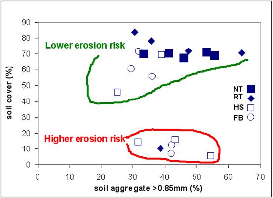
The susceptibility of each individual plot to wind erosion in the 2004-05 drought is shown in Figure 9 below. The plots fall into two distinct groups for erosion risk: high erosion risk and the low erosion risk. Six plots are classified as being a high erosion risk, comprising three from Hungry Sheep, two from Fuel Burners and one from Reduced Till. 

Figure 8: Soil transport rate Q (g/m/s) for each of five plots in the four farming systems, as assessed in 2004-05 drought (BCG 2006)

Figure 9: Individual system plots’ susceptibility to erosion based on soil aggregates (% > 0.85mm) and soil cover (%) (BCG 2006)

 

3.3 Profitability

Gross margins

In Table 9 is shown the average activity gross margin for each paddock and system under study. The paddock average gross margin is the average gross margins for that paddock over the six years of the trial in GM/ha/yr. The system average is the average of the paddock average gross margins.  The complete set of gross margins for each system are shown in Appendix 4. The Reduced Till system had the highest average gross margin per hectare per year of $80.71/ha followed by Hungry Sheep, Fuel Burners and No Till with respective gross margins of $79.81/ha, $76.44/ha and $32.59/ha. The paddock average GM/ha/yr range for each system was:

• No Till: -$12.54 to $84.26/ha;
• Reduced Till: $14.57 to $157.81/ha;
• Fuel Burners: $48.81 to $108.18/ha; and
• Hungry Sheep: $16.69 to $194.92/ha. 

Table 9: Total and average paddock gross margins per hectare for the farming systems in the trial.

* Average GM/ha/yr (Gross Margin/hectare/year) for each paddock from 2000 to 2005 (6 years).

^ Average GM/ha of each cropping system from 2000 to 2005.

 

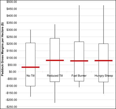
In Figure 10 the variability in gross margins is shown for 30 gross margin measurements (six years by five plots per system) across each of the systems from 2000 to 2005. Each box is representative of the middle 50 percent of every gross margin for that system. The upper and lower stems respectively show the top and bottom 25 percent of the gross margins realised by each system.

Figure 10: Stem and box plot chart depicting the individual paddock gross margins for each system over the life of the project from 2000-2005.

 

Examining the products, income and variable costs of the gross margins identifies areas of strength or weakness. Figure 11 is a chart that shows the annual income and variable costs for each system spanning the life of the project. 

Figure 11: Annual average income and variable costs for each system over the life of the project from 2000 to 2005

 

 

Annuity and net present value

Table 10 below shows the NPV, Annuity and average annuity per hectare for each paddock and respective farming system based on a 5% interest rate. As with the average gross margins the Reduced Till system has the highest annuity of $84.08 followed by Hungry Sheep ($82.16), Fuel Burners ($80.00) and No Till ($32.06) 

Table 10: Net present value for 6 years, and annuity values, of the activity gross margins per hectare for the farming systems in the trial.

Sensitivity

Table 11 below outlines the sensitivity of each of the systems to changes in yield, grain/seed price, inputs, sheep price, wool price, agistment price and sheep inputs.  The upside and downside changes are based on a 10% positive and negative change in the aforementioned sensitivity factors. Some sensitivity factors are not included in some systems and as such provide no changes in gross margin and are therefore excluded.

Table 11: Sensitivity of system average gross margin per hectare per year to 10 percent changes in yield, returns and costs

4. Discussion

The aim of this investigation was to determine the profitability and sustainability of different cropping systems in the Wimmera/Mallee. It is important to analyse the results beyond the primary outcomes and explore the contributing factors.

4.1 System profitability/gross margins

As an indicator of the relative merit of each system the gross margins serve a useful purpose. It is important that each system be compared on an equal basis. It was important for each system to have completed at least one cycle of its rotations. The six-year period over which the analysis has occurred has provided sufficient time for this to occur. In addition, the ‘phase confounded’ trial design also improved the ability to make fair comparisons. As Makeham and Malcolm (1998) put it:

If comparing the profitability of different farm plans involving different crop and livestock combinations, returns from whole sequences are compared, not single segments of a sequence. If it is assumed that each segment of each sequence were going to be present on the farm in each year then the annual total gross margin per sequence-hectare is the figure to use to compare with alternative rotations (p.188).

It is evident from the results that three of the systems, Reduced Till, Fuel Burners and Hungry Sheep, have performed at a similar level over the six year period, with only $4.27/ha separating the ‘across paddocks’ average annual gross margins. This is an insignificant difference when it is juxtaposed with the $80.71/ha average annual gross margin achieved by Reduced Till, the most successful of the three, (Hungry Sheep and Fuel Burners achieved $79.54/ha and  $76.44/ha respectively). The poorest performer was the No Till system, with an average annual gross margin of $32.59/ha.

When considering the NPV and respective annuity the results are relatively unchanged when compared to the average annual gross margin, with the Reduced Till having the highest followed by Hungry Sheep, Fuel Burners and No Till. Calculation of the annuity of each system does not alter the results with the same three systems remaining relatively close and the No Till system still substantially lower. Given the prevailing climatic and environmental conditions over the six-year period, the Reduced Till, Fuel Burners and Hungry Sheep systems were the most profitable.

The results shown in Table 9 and 10, and Figure 10, form the basis for comparison and judgement about the relative economic merits of the alternative farming systems. Each system recorded performances considerably above and below the mean in some paddocks. Looking at Figure 10, it is evident that Reduced Till had a mean economic performance similar to Fuel Burner and Hungry Sheep, but also had a greater ’down-side’ risk, with paddocks that lost the largest amounts of money in some years. Conversely, paddocks under Fuel Burner and Hungry Sheep produced the lowest losses in the poor years and, significantly, achieved the highest gross margins by a considerable margin in the good years. On average the Reduced Till, Fuel Burner and Hungry sheep achieved about the same results, all better than No Till. Fuel Burner was the least volatile system, closely followed by Hungry Sheep.

The climatic conditions that prevailed over the period need to be appreciated. Rainfall over the six years was significantly lower than the 100 year average. Conditions at the site are described in Table 1. The long-term average annual rainfall and growing season rainfall were reached only in 2000, and then only GSR deciles five and six respectively were reached.  Of the remaining five years, two were very poor with GSR deciles of one in the year 2002 and two in 2004. The other three years, 2001, 2003 and 2005, were poor years with GSR deciles of three. Such conditions make it difficult for any farming system to be profitable or environmentally benign. The possibility must be considered that the No Till system could perform similarly to the other systems under quite different, better, climatic conditions.

In addition to the climatic conditions, the soils at the site also have to be considered.  According to the BCG (2006):

The systems site is regarded as a site with severe subsoil limitations …It is generally regarded that EC values above 0.8ds/m, ESP above 19%, chloride levels above 800mg/kg, and boron above 15mg/kg inhibits root development, reduces water uptake and affects plant growth. These critical values generally apply to cereals such as wheat and barley. Canola and pulses are much more sensitive to subsoil constraints (BCG, 2006)

When these critical levels exist, soil type will restrict crop growth. The electrical conductivity and chloride levels generally begin to present a problem within the 50 to 70 cm soil depth range. While having an affect on the potential crop growth, this becomes a relatively minor consideration when compared to the exchangeable sodium percentage and the boron levels that become toxic in the 10 to 30cm soil depth range. The full soil test results can be found in Appendix 1.

The amount of boron present in the soil at the site is considered to be among the highest concentrations in Australia.  This will no doubt have an effect on the potential yield of some crops. The relatively poor gross margins achieved by the No Till system may be a result of these extreme soil conditions. It may be that the other three systems have the ability to perform better than the No Till system under the prevailing soil conditions.  The gross margin results may differ under soil conditions more suited to the No Till system.

Over the term of the trial, the relative equality of the most successful three systems (Reduced Till, Fuel Burners and Hungry Sheep) in their average gross margins is derived from their having similar income and variable cost levels. None of the systems is distinct from the others by a combination of high returns combined with high costs, or lower returns with low costs. In terms of profitability, it is difficult to separate them. 

As suggested in Figure 11, the No Till system performed poorly in relation to income. In most years, and on average, this system had the lowest income primarily as a result of poor yields. Compounding this problem, the No Till system showed the highest average variable costs across the project term. This is likely to be due to the system’s high reliance on expensive chemicals for weed control.  The perceived benefits from this system - increased amounts of organic matter and, as a consequence, improved soil structure - do not appear to be reflected in the system returns, possibly due to the poor climatic and soil environment.  Despite the reduction in fertiliser costs due to the increased organic matter, it is evident that, for this system to become more successful under these conditions, it is necessary for chemical costs to be reduced.  It appears that the use of cultivation or sheep, which are used in the other systems, has the ability to provide a significant benefit in controlling weeds without compromising the level of variable costs. 

4.2 Sensitivity of the systems

To further analyse the potential profitability and relative robustness of the systems, the sensitivity was measured to changes in a number of factors including grain prices, input prices and sheep returns and inputs. The sensitivities have been calculated both in terms of dollar values and as a percentage change away from the existing average gross margin. These are shown in Table 11 above. Each system is most sensitive to yield, followed by grain and input prices. The sheep-related sensitivity factors have a minimal impact on all of the systems.

In percentage terms, the No Till system is most sensitive to changes. This system has the largest upside and downside movements across the three major sensitivity factors with a range of ±43.5% to ±56.6%.  This is substantially higher than the range of the other three systems which was ±14.6% to ±28.3%. The high percentage changes of the No Till system are not surprising given the relatively small gross margins achieved. When movements in aggregate dollars are compared, with the exception of inputs, this system has the smallest movements.  One explanation for the small dollar value movements for yield and grain price is due to the  system having the smallest yields. In reality, this system compared to the other three most likely has the greatest capacity to expand its yields as it is starting from a much lower base. 

Despite the dissimilarity in production methods between the three remaining systems, Reduced Till, Fuel Burners and Hungry Sheep, the income, variable costs and gross margins of these systems are very similar.  When changes in the sensitivity factors are tested, the performance of these three systems tracks each other closely. There are some small differences that could benefit one system over another given certain changes. 

The Hungry Sheep system is the most diversified of the systems in the trial with a significant portion of the income derived from sheep.  This decreases the reliance of the system on cropping and creates smaller movements in the gross margins when the cropping sensitivity factors are altered. The system therefore provides some downside protection when compared with the other systems, but may be restricted if grain prices or yields increase above the increases in inputs.  Another advantage of this diversity is that some of the costs are spread. If the cropping costs increase, the overall cost increases may be contained due to the separation of sheep costs.

The gross margins from the Reduced Till and Fuel Burner systems moved similarly as the levels of the key variables changed.. The Reduced Till system was slightly more responsive in the yield and grain price sensitivities. This is because of the higher yields achieved by this system allowing it to be more responsive to changes.  The advantage of the Fuel Burner system is that it has the potential to increase further than other systems with positive changes in yield and price. This is a likely outcome given the current economic and climatic conditions. 

4.3 System gross margin variation

An average gross margin across all years and paddocks does not take into consideration the range or variation of gross margins of a given system. Figure 10 represents the performance of each system over the trial period. This shows that certain systems have a greater degree of variation in gross margin over the period compared with the others.  A farmer’s tolerance to risk or income fluctuation will be a contributing factor in determining the farming system applied.  From Figure 10 it can be seen that a risk-averse farmer will likely choose to use the Fuel Burner system. While this system produced the second greatest number of negative gross margins (17), the losses were controlled. This is because of  the relatively low levels of variable costs associated with this system.  It is also evident from Figure 10 that the ability of the Fuel Burner system to control losses did not occur at the cost of creating high gross margins. This system achieved a number of gross margins in excess of $400/ha. 

The Hungry Sheep system also provides a producer with income stability over the period. This system limited the number of negative gross margins to 13. This was also achieved by the Reduced Till system, but the size of the losses experienced by the Reduced Till system were substantially larger than those of Hungry Sheep.  Another advantage the Hungry Sheep system has over Fuel Burners is that some paddocks still had the potential to perform strongly, achieving gross margins in excess of $360/ha.  However, despite not having the high gross margins, the Reduced Till system had the same number of negative gross margins as Hungry Sheep, albeit slightly larger, and more consistently achieved positive gross margins.  This system’s top gross margins (25% of the total gross margins) fell within $100/ha of each other between $240/ha and $340/ha. 

Over the trial period, the No Till system provided farmers with the least amount of protection from losses and the smallest potential for high gross margins. With 18 negative gross margins and the highest positive gross margin at $300/ha, this system did not perform well over the trial period. It is evident from Figure 10 that this system was substantially inferior to the others.

Despite the Hungry Sheep system providing sound income stability, it should be noted that the majority of the systems’ poorest gross margins resulted from pasture crops where sheep are included in the gross margin.  The poor gross margins from the pasture crops was not due to a lack of income but was a result of high costs, particularly the cost of feeding the sheep. Exposure to, and management of, livestock-related drought risk matters. In a number of cases the cost of feeding the sheep well outweighed the income that they derived. Should the number of sheep be reduced in dry years, gross margins associated with the sheep could be significantly improved.  When there are indications of dry year the decision to sell the sheep needs to be made earlier.  This may be at the cost of reduced income if the season were to change. It would help to significantly improve the downside protection offered by this system  and help to maintain cashflows.

4.4 Sustainability of the systems

The previous analysis has focused on the profitability of each of the systems. The success and longevity of a system relies not only on short term profitability; it is also imperative that it be technically and economically sustainable in the medium and longer terms.  The sustainability indicators showed minimal differences in technical sustainability between the four systems. The indicator that provided the greatest difference between systems was the risk from wind erosion.  The lack of difference in technical sustainability between systems is most likely because of the climatic conditions over the trial period.  The soil microbes, weeds and soil-borne diseases that were tested flourish under moist conditions. Such conditions did not happen. The rainfall over the period was substantially below the long-term average.  The poor growing conditions for these organisms prevented them from establishing themselves or building up in any one system. An additional consequence of the poor seasons is a tendency towards less crop biomass production, enabling a faster breakdown of the crop residue post harvest.  The crop residue acts as a vector for a large number of soil organisms. The reduced amount of crop residue prevents the build up of both soil-borne diseases and beneficial soil microbes.  To further assess the effect of each system on these sustainability indicators, improved climatic conditions may need to exist.

The poor climatic conditions over the trial period have enabled some differentiation to be discerned in relation to wind erosion risk.  The lack of biomass in the crops also reduces the amount of soil cover for each system, exposing them to a greater level of wind erosion risk.    It is generally considered that a paddock with 40% stubble coverage is safe from wind erosion. If this is the case, it is evident from Figure 7 that all systems in the 2002-03 drought were at risk.  Some, however, were more so than others. The No Till system provided the best protection, with a minimum coverage of stubble of 30%.  The remaining three systems retained stock in at least one of their paddocks throughout the season. This, in conjunction with tillage operations, significantly reduced the soil coverage.  This is evident in Figure 7, as shown by the distinct reductions in soil cover over the three assessments.  The Hungry Sheep system provided the least amount of erosion protection with only 7% cover at the time of the third assessment. This level of cover was low, making the paddocks susceptible to erosion.  The comparatively high stocking rate of this system creates a significant disadvantage in this sustainability indicator. To lessen this problem, stocking rates would have to be reduced during the poor seasons. The final coverage of Fuel Burners and Reduced Till of 15%, while still at risk, provides more protection than the Hungry Sheep system.

A similar outcome resulted during the 2004-05 drought.  The No Till system performed well by this indicator, providing good protection from soil transport, as identified in Figure 8.  As outlined in the results, the Hungry Sheep, Fuel Burners and Reduced Till systems had paddocks with a moderate risk of wind erosion.  Figure 9 illustrates a similar outcome to Figure 8 with 6 plots at risk of wind erosion.  It should be noted that the Reduced Till system significantly improved in 2004-05 compared to the 2002-03 drought, having only one paddock at risk in 2004-05.  As was the case in the 2002-03, Hungry Sheep and Fuel Burners still produced a significant level of susceptibility in 2004-05. Again Hungry Sheep provided the greatest level of susceptibility with three paddocks at high risk and one paddock at the more susceptible end of the low risk paddocks. Sheep utilisation and increased tillage increased the danger of wind erosion.  Possibly, stock should be sold earlier, or tillage operations reduced. Unfortunately, this may occur at the cost of a superior gross margin.

Although not covered in the results, the type of soil cover on a paddock also had a significant impact on the susceptibility to wind erosion.  The standing stubble in the No-till and Reduced Till systems provided significantly better protection than the Hungry Sheep and Fuel Burner systems that incorporated sheep and tillage. 

4.5 Non-economic considerations

As well as assessing the profitability and sustainability of systems in the Wimmera/Mallee, non-economic issues also matter. These inevitably affect the choices that a farmer will make about crop systems. Farmers have different preferences when it comes to the work to be done on a farm.  A farmer may have an aversion to a specific aspect of a particular system. A common element that influences system decision is the inclusion of livestock, in this case, sheep.  The nature of sheep husbandry often requires regular observation, which may interfere with a lifestyle desirable to a farmer.

A system that incorporates sheep will require a farmer to be present on the property more often: sheep work can often monopolize weekends or prevent a farmer from taking a holiday. Conversely, a cropping system which does not incorporate grazing does not require the farmer to be consistently on site; it can be managed from afar or can allow for off-farm activities including additional employment, a supplementary business or holidays.  Another influence on the inclusion of sheep in a system is the extra infrastructure that is required. A sheep system will require shearing sheds, yards, laneways and adequate fencing.

Other considerations that may influence a farmer’s decision may be an aversion to tractor work.  Increased tractor hours may be a sufficient deterrent to the adoption of a given system. Conversely, farmers may enjoy tractor work or have a love for machinery which may influence their system choices.

Perhaps the most significant non-economic consideration is a farmer’s acceptance of, or aversion to, risk. People have different tolerance levels in dealing with the potential for a severe loss.  A system that experiences significant losses in some seasons and is not diversified – one in which income only comes from one operation – may not be suitable for a person averse to risk.  It is evident from Figure 10 that a risk-averse farmer would probably choose Fuel Burners because of the protection from the worst outcomes that it offers, or Hungry Sheep with its level of diversification and the potential for earning income from grazing and stabilizing total income. The agistment in the Reduced Till and Fuel Burner systems does not provide sufficient income to provide diversification and reduce risk.

5. Conclusion

Long-term farming systems trails are relatively uncommon in Australia, particularly those which consider the economic implications of agronomic farming systems and include a livestock component.  The Birchip trial, which incorporates both of these factors, provides a relatively rare opportunity to compare the profitability and sustainability of four distinct farming systems in the Wimmera and Mallee. It has produced some interesting outcomes, though as yet they are not entirely conclusive. 

Three of the four systems, Reduced Till, Hungry Sheep and Fuel Burners, have performed comparably, producing similar profitability outcomes well above the level of the fourth system, No Till. The No Till system underperformed in terms of profitability when all paddocks are looked at, over a period of low rainfall, when compared with the remaining three systems.  Hungry Sheep and Fuel Burners were the least volatile of the systems, and had the lowest ‘poor’ performance and the highest ‘good’ performances. The similarity of economic performance over the run of years means that definitive conclusions about which is the best system for particular farms in the region must, as ever, be made on a case by case basis. The economic information forms part of the information that goes into decisions about which system to adopt. The lack of clear economic differentiation between systems may be in part a result of the poor climatic and soil conditions experienced at the site over the term of the trial. Still, that is Mallee farming - for some of the time. Results from the trial after a few good years would be instructive too.

With the exception of risk from wind erosion, the trial provided little evidence of differentiation between the four systems in sustainability terms.  The No Till system provided substantial wind erosion protection followed by Reduced Till which provided acceptable protection. The Fuel Burners and Hungry Sheep system did not provide adequate protection and were vulnerable in the drought periods of 2002-03 and 2004-05.

The sensitivity of each of the systems to changes in the core factors revealed the robustness of the Hungry Sheep system relative to the other three systems. The diversification of income sources associated with this system provides additional downside protection from changes in any one factor. Although only a small portion of income is derived from sheep, it reduces the pressure on cropping returns. This creates a significant advantage to the Hungry Sheep over the other systems in providing significant risk diversification.

A farmer’s tolerance to risk or income fluctuation will be a contributing factor in determining the farming system applied.  The downside gross margin protection offered by the Fuel Burner and Hungry Sheep systems may encourage a risk-averse farmer to adopt that system. Despite receiving the highest average gross margin, the Reduced Till system did not provide the same level of protection. This is a consideration that a farmer would need to take into account when adopting any given system.

The profitability and sustainability outcomes realised by the Hungry Sheep system throughout the trial indicate that livestock can play a significant role in a cropping system in the Wimmera and Mallee. In what can be considered tough seasonal conditions, the Hungry Sheep system managed to compete with the other systems in terms of profitability. However, under the drought conditions, the sheep incorporated into the system created a risk of wind erosion that may impact on its technical sustainability and future profitability. This problem might have been avoided if the decision to sell off sheep earlier in the season had been implemented at an early stage in adverse conditions. Though this may result in missed income if the season turns around it would help to ensure the viability of that system in the future. Given the climatic conditions during the duration of the study, the decision to sell off sheep earlier would have been  beneficial for the Hungry Sheep system.

There is not one crop farming system that is superior in terms of profitability and sustainability. Each system has strengths and weaknesses. Given the adversity of the farming conditions in the period during which the trial was undertaken, it seems reasonable to speculate that better seasons may have led to greater differentiation between the systems in technical and economic outcomes. Continuing the trial for some years may  produce robust conclusions.

6. Acknowledgements

Fiona Best and other staff at the Birchip Cropping Group were always willing to respond promptly to requests for information.  For this we are extremely grateful and we thank them for the support they have given over the last year. 

Tim McClelland’s employer Mr Shane Kelly, Managing Director of Adviser Edge Investment Research willingly gave time for the research to be done.

7. References

Armstrong, R. (2005). "Farming Systems Program."  Retrieved 18/4, 2006.

BCG (2006). 2005 Season Crop and Pasture Production Manual, Members Only Edition. Birchip Cropping Group. B. C. Group. Birchip, Birchip Cropping Group.

BCG (2006). Six Seasons of the BCG Farming Systems Trial. Birchip Cropping Group. B. C. Group. Birchip, Birchip Cropping Group.

BISShrapnel, 2006. Long Term Forecasts Australia, 2006-2021, 32nd edition. Long Term Forecasts. BIS Shrapnel, Melbourne.

BOM (2006). Birchip Post Office Climate averages, Bureau of Meteorology.

BOM. (2006). "Climate Averages for Australian Sites."  Retrieved 5/9, 2006.

Cawood, R., R. Chechet, et al. (1996). Climate, Temperature and Crop Production in South-eastern Australian. Horsham, Victorian Institute for Dryland Agriculture.

Elliot, M., 1996. Sheep Production. Richard Lee Publishing, Castlemaine.

Gerik, T. and D. Freebairn (2004). Management of extensive farming systems for drought-prone environments in North America and Australia. New directions for a diverse planet - The 4th International Crop Science Congress, Brisbane.

Glendinning, J. S. (2003). Australian Soil Fertility Manual. Collingwood, CSIRO Publishing.

Hannah, M. C. and G. J. O'Leary (1995). "Wheat yield response to rainfall in a long-term multi-rotational experiment in the Victorian Wimmera." Australian Journal of Experimental Agriculture 35: 951-60.

Heenan, D. P., A. C. Taylor, et al. (1994). "Long Term Effects of Rotation, Tillage and Stubble Management on Wheat Production in Southern N.S.W." Australian Journal of Agricultural Research 45: 93-117.

Hulugalle, N. R., P. C. Entwistle, et al. (2002). "Cotton-based rotation systems on a sodic Vertosol under irrigation: effects on soil quality and profitability." Australian Journal of Experimental Agriculture (42): 341-349.

Jochinke, D., N. Wachsmann, et al. (2003). "Soil Water availability determines optimum sowing rates for safflower in southern Australia."  Retrieved 8 September, 2006.

Knopke, P., V. O'Donnell, et al. (2000). Productivity Growth in the Australian Grains Industry. T. A. B. o. A. a. R. E. (ABARE) and G. R. a. R. a. D. C. (GRDC). Canberra, ABARE.

Leys, J.F., Semple, W.S., Raupach, M.R., Findlater, P., Hamilton, G.J., 2002. Measurment of size distributions of dry soil aggregates. Soil Physical measurements and interpretation for land evaluation.

NSWDPI, 2006. Gross Margins. p. 3 pages.

Makeham, J. P. and L. R. Malcolm (1998). The Farming Game Now. Melbourne, Cambridge University Press.

NSWDPI, 2006. Gross Margins. p. 3 pages.

Patterson, H. D. (1964). "Theory of cyclic rotation experiments." J. Roy. Stat. Soc. 26: 1-45.

Pechey, L. (2006). Agriculture in Australia - Past, Present and Future. T. A. B. o. A. a. R. E. (ABARE). Canberra, ABARE.

Pilkington, L. J. (2006). Core Site - 2005. CWFS Research Compendium 2005-06. C. W. F. S. (CWFS). Condobolin, Central West Farming Systems: 17-24.

Pratley, J. E. and D. L. Rowell (1987). "From the first fleet - Evolution of Australian farming systems." Australian Society of Agronomy Monographs: 2-23.

Prior, R. B. M., J. Which, et al. (2003). Combining biophysical and price simulations to assess the economics of long-term crop rotations. Australian Agricultural and Resource Economics Society Conference, Fremantle, Muresk Institute of Agriculture.

Rodriguez, D., J. Nuttalll, et al. (2006). "Impact of subsoil constraints on wheat and gross margin on fine-textured soils of the southern Victorian Mallee." Australian Journal of Agricultural Research (57): 355-365.

SCA (1991). Sustainable Agriculture. SCA Technical Report 36. Melbourne, Standing Committee on Agriculture.

Schultz, J. E. (1995). "Crop production in a rotational trial at Tarlee, South Australia." Australian Journal of Experimental Agriculture 35: 865-76.

So, H. B., R. C. Dalal, et al. (1999). Potential of Conservation Tillage to Reduce Carbon Dioxide Emission in Australian Soils. 10th International Soil Conservation Organisation Meeting, West Lafayette.

Squires, V. and P. Tow (1991). Dryland Farming, a systems approach, an analysis of dryland agriculture in Australia. Sydney, Sydney University Press.