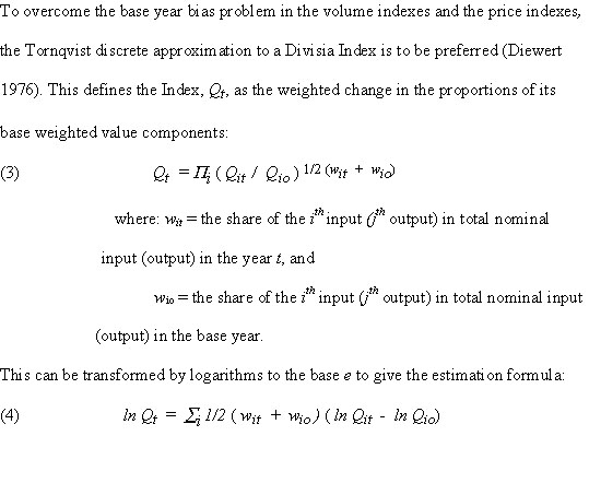
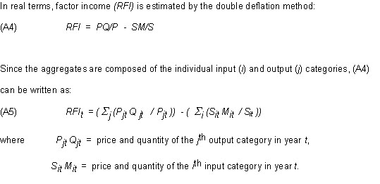
Agribusiness Review - Vol. 9 - 2001

Paper 1
ISSN 1442-6951

Recent Trends in New Zealand Agricultural Productivity

Rod Forbes and Robin Johnson
Ministry of Agriculture, Wellington and Consultant, Wellington, respectively ¹.

1 Comments of a referee are acknowledged. Paper first presented at the 44th Annual Conference of AARES at Sydney, January 2000.

Introduction

This paper discusses trends in New Zealand agricultural productivity at the farm level since 1972. Total input and factor input measures of productivity are derived and discussed. The method is based on Tornqvist (1936) index numbers which weight changes in the output and input mix as an average between base year weights and current year weights. Comparisons are made with base year weighting systems (Laspeyre Index Numbers) that are derived from Statistics New Zealand (SNZ) data sets available at the time of analysis. However, from September 2000 quarter, SNZ have adopted a chain link system for their national accounts.

It is clear that resources will move out of an industry if relative returns to those resources are not maintained. In agriculture, this involves the inputs that producers buy from elsewhere, the land and capital used for productive purposes, and the producer's (and family's) own labour. By and large, if returns to a producer is deemed unsatisfactory in terms of existing production systems and market prices, the producer's response is either to change systems of production, or economise on the use of inputs, or sell up.

The level of return to farming is determined in turn by market opportunities, domestic and overseas, and by the level of efficiency in the use of the basic resources available. In the New Zealand situation where the majority of farm products are exported, it is the international terms of trade between primary product prices and farm input prices, which is the most important determining factor.

In general terms, the terms of trade for primary products and thus farmers have trended downwards since World War II (Tyers and Anderson 1986). Yet farm incomes have largely been maintained and resources have not moved out of the farm sector. The reason for this is the rise in efficiency in the use of resources over the long haul. The latter is reflected in the measures of productivity described in this paper.

In general terms, the rise in productivity has tended to largely cancel the effects of declining terms of trade on farm incomes in the agricultural sector in New Zealand in the period since the second world war. The paper discusses the relative size of the agricultural sector in New Zealand and the main trends in production, resources and resource use since 1972. This includes a discussion of how best to measure changes in farm productivity. (An appendix sets out the production theory that is involved). Finally we return to the role of the terms of trade and productivity in maintaining farm level incomes over recent decades.

The Agricultural Sector in New Zealand

We define the agricultural sector in the same terms as the national income accounts prepared by SNZ (1999a). The sector account for agriculture includes all farm production activities for both home consumption and market purposes, contracting activities to other farmers and income from farm-owned forest plots. All products are valued at the point of first sale including accumulated stocks. For productivity analysis, gross revenues, capital resources and purchased inputs are deflated by appropriate index numbers of prices.

National income or gross domestic product (GDP) for the sector is derived by subtracting the cost of purchased inputs from gross revenue. GDP is the residual amount left to pay the rewards of paid and unpaid labour, depreciation of capital assets and the cost of borrowing. It is thus the net return available to reward the factors of production, capital and labour.

The Standard National Accounts approach (SNA) divides factor income (GDP) into rewards to paid labour, consumption of capital (depreciation), operating surplus plus a correction for subsidies and taxes. As there is no published share for the reward to all labour, this has to be estimated. SNA gives the wage labour component as a "paid" reward and attributes the reward to owner's labour to operating surplus. To separate the components appropriately, we estimate capital costs first and make wage rewards and equity rewards a residual. The total cost of capital is estimated as the sum of depreciation of total capital and the service cost of borrowed capital (see appendix).

The factor share of labour varies considerably by this method over a period of time (Figure 1). The share to the service cost of capital mirrors the way monetary policy affected interest rates paid by farmers in the period concerned. The freeing up of the economy from 1984 led to historically high, new mortgage interest rates between 1986 (19.1%) and 1988 (18.9%). Rates fell steadily to 7.9% in 1994 and then rose to remain slightly above 10% between 1995 and 1998.

Figure 1: Disposition of nominal agricultural GDP

Trends in Factor Income in Farming and the Terms of Trade

Althought the absolute level of GDP in agriculture has been rising over the last 30 years, the relative proportion of total national income has slowly declined. Expressed in terms of nominal GDP per person employed (FTEs), a more serious decline is evident (Figure 2). Agricultural producers always complain of the low incomes they receive and these statistics indicate how much in national income terms. Up to 1980, farmers earned comparable incomes in nominal GDP per person employed terms to the rest of the economy. Since that time, there has been a consistent deterioration in relative incomes. Two factors stand out, the economic reforms from 1984 and commodity terms of trade.

Figure 2: Nominal GDP per head

Prior to 1980, a regime of producer support and a fixed exchange rate appears to have kept relative prices stable between the farm sector and the rest of the economy. The main determinant of changes in farming incomes is the commodity terms of trade. Farmers are at the mercy of international commodity price trends, modified by changes in the exchange rate and the competitive structure in the value added chain between farm gate and FOB. The impact on farm incomes can be judged by a comparison of the general [implicit] prices which go to make up national GDP values and the [implicit] prices that make up farm GDP (Figure 3). From 1980, farm level GDP prices have lagged well behind national GDP prices. This is because farm product prices and input prices are largely determined by trade returns and not internal demand. As a result, especially in the period 1985 onwards, the tradeable sector was open to international economic forces while the non-tradeable sector remained shielded from international price competitiveness.

Structural adjustments within the agricultural sector have taken place in response to the reforms since 1984 and have improved the relative returns to farming compared with what they would have been. Economic farm sizes have steadily increased along with the shedding of farm labour and an increasing reliance on off-farm income. At the same time, there has been an increase in subdivison in some areas into lifestyle blocks, with the consequent lowering of agricultural production. The major policy interest in agricultural productivity is whether the rate of change has increased with the deregulation of farming in the last 20 years. A major political-economic paradigm shift occurred in 1984 with the election of a Labour Government with free market tendencies. A mini-Budget in December 1984 cancelled government subsidy support to the agricultural sector and the NZ dollar was allowed to freely float from March 1985. We thus chose a break point of March 1985, for a pre and post reform comparison of growth rates in the productivity indexes derived.

Productivity Analysis

Two productivity ratios are derived in this paper; total input productivity and total factor productivity. Total input productivity (TIP) is a ratio of gross output to the combined inputs of materials, labour and capital; total factor productivity (TFP) is the ratio of net output (real GDP) to the combined inputs of labour and capital.

In line with the SNA conventions (Statistics New Zealand 1996), nominal gross value of production is deflated, product by product, by price indexes of products sold at first point of sale and re-aggregated; nominal material inputs (intermediate consumption), input by input, by price indexes of inputs at point of sale and re-aggregated, and real GDP (factor income) is determined by difference.

The measure of real labour input is based on estimates of fulltime equivalents employed with appropriate weights for part-time employees (Philpott 1994). The definition of the physical capital employed is based on estimates of the stock of assets curently held by farmers in the aggregate. Philpott (1994, 1995, 1999a) provides two series of capital stocks: one derived from business depreciation rates (‘net capital stocks') and one from a vintage model where "disappearance" is estimated for whole blocks of assets on a systematic basis (‘gross capital stocks'). Philpott's gross capital stocks tend to be 50 per cent higher than his net capital stocks. The gross series is used in this study as it indicates more closely the actual stock employed rather than some book-depreciated set of assets. Capital stocks are derived from a perpetual inventory model (see appendix).

These conventions provide consistent time series of real gross output, real intermediate input, real net output, labour employed, and capital stock employed. Since the real national income data used is essentially base year price-weighted (see appendix) the resulting data series, by definition, are Laspeyre indexes of gross output, intermediate input and net output (Figure 4).

Labour employed in agriculture reached a peak in 1981-82 and has since declined slowly. Capital employed (on a gross basis) increased steadily until 1985-86 and then slowly declined also. [Put another way, the additions to the stock (investment) were smaller than the losses due to obsolescence]. In terms of the single productivity ratios (Figure 5) for labour and capital, there has been a 2.2 times increase in net output per FTE since 1972 and a 1.8 times increase in net output per unit of capital. Total factor productivity will be the weighted average of the two. The objective of the present paper is to derive suitable weighting systems for a combined labour and capital productivity index (total factor productivity) and for a total input productivity index.

The Laspeyre factor income productivity ration (TFP) can be defined as:

TFP_t = (P₀ Q_t - S₀ M_t) / (W₀ L_t + R₀ K_t)        (1)

where P₀, S₀, W₀, R₀ are the prices for the base year
Q_t = quantity of gross output
M_t = quantity of material inputs
L_t = quantity of labout inputs
K_t = quantity of capital inputs

The Laspeyre total input productivity ratio (TIP) may also be defined in the same way:

TIP_t = (P₀ Q_t ) / (W₀ L_t + R₀ K_t + - S₀ M_t)        (2)

These productivity ratios are the respective base years of the Laspeyres Index Number. If the base year ratios are set equal to 1000, changes in the productivity ratios in all other years are represented by indexes.

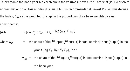
By taking anti-logs, the base year takes on a value of unity. The resulting index numbers now represent a moving weighted average of base year input (output) values and the current input (output) values.

Tornqvist weighting is used to overcome biases caused by changes in the respective weights of the components of a given volume index. In the case of intermediate inputs, for example, the use of fertiliser may be changing systematically during the period of observation. Base year weights of different inputs would freeze the true weighting over a period of time. Similarly for the total fertiliser index of volume - a base year weight would freeze the mix of different fertilisers when farmers were changing their respective mixes. These biases can thus arise from any change of use in a productive input and are commonly found in fertilisers, weedkillers, sprays, and other inputs. The same reasoning applies to changes in the mix of outputs.

The analysis provides appropriately weighted index numbers of gross output, intermediate inputs and factor inputs (labour and capital). For the TIP estimation we use gross output/weighted sum of intermediate and factor inputs. For the TFP estimation, we derive net output by converting back to real dollar values and subtracting intermediate inputs from gross output and then convert back to an index number, and then estimate TFP from the ratio net output/weighted factor inputs.

ln TFP_t = a + b T       (5)

Where TFP = index numbers representing total factor productivity
a = a constant
b = regression coefficient representing the rate of growth
T = time in years elapsed

We first consider the effect of the different weighting systems. Figure 6 shows a comparison of the two weighting methods for gross output of the agricultural sector; Figure 7 shows the comparison for total inputs employed. In general, the Tornqvist method tends to lower the estimate of weighted output and weighted total input compared with base year weighting in the latter years. We suggest that higher value attributes of each aggregate are given less weighting by the Tornqvist method in these years.

Table 1 shows total input productivity (TIP) growth rates estimated by Laspeyre base-weighted method and by the Tornqvist geometric average weighted method. The latter weights are derived from average value shares between the current year nominal factor shares and the base year factor shares (1982-83). If an input or an output mix is changing in a systematic way the geometric average method is the preferred method. Figure 8 shows the two indexes.

Table 1: Total input productivity by weighting method and periods (growth rates %)

Total input productivity tends to be over-stated by base-weighted indexes in all periods though not by a high margin. Higher output growth is matched by higher input growth though in the sub-periods, the fitted line is not always consistent. The better estimate of long run total input productivity is thus 1.5% per year since 1972. Both methods suggest that the rate of growth has improved by a considerable margin since 1985 compared with the earlier period 1972-84.

Table 2 shows the same results for total factor productivity and Figure 9 shows a comparison of the two weighting methods for the total factor productivity (TFP) index.

Table 2: Total factor productivity by periods (growth rates %)

Again Tornqvist indexes tend to lower the factor income increase and the factor input increase (slightly) with the resulting effect on the productivity growth rate. Because intermediate inputs (deleted from this comparison) grew at a lower rate than total output, the rate of growth of factor income is higher than that of total output (as in Table 1). Thus the best estimate for factor productivity growth for the period since 1972 is 3.5% per year rather than 4.1% per year as might have been indicated by the Laspeyre index. It is clear that there was an acceleration in TFP in the period since 1985.

Comparative Results

Diewert and Lawrence (1999) estimate the rate of growth of factor productivity in agriculture for the period 1978 to 1998 as 3.87% per year. For more careful comparision we need to look at the specification of their model:

"To form separate TFP indexes for the 20 industries we now take real production GDP as output, normalise it to equal 1 in 1978, and form a chained Fisher index of the three industry inputs - labour hours, plant and equipment stocks, and building and construction stocks - using labour costs and capital user costs as weights. We then take the ratio of the industry's total output to total input index to form the industry's TFP index. The industry TFP indexes use our preferred base case specification of production base GDP, the database's composite labour series, and our net capital estimates".

The chained Fisher index gives very similar results to the Tornqvist index – the Fisher index being the geometric average of the Paasche and Laspeyre indexes. Production based GDP is the same as used above; the use of labour hours tends to increase the input of labour and decrease the resulting TFP compared with FTEs; and the net capital stock [derived from the Philpott papers] grows more slowly than the gross capital stock used by ourselves. Thus the Diewert and Lawrence TFP estimates are lower by reason of their labour definition but higher by reason of their capital definition. Our series also extend over a longer period (1972-98) and hence contain more information than that of Diewert and Laurence. A summary of their sector estimates of industry TFP growth by their methodology is shown in Table 3.

Table 3: TFP's by Diewert and Lawrence (1978-98)(growth rates %)

The particular reasons for the growth or lack of growth in each sector needs to be examined against the background of labour and capital input changes, the uptake of technology, and other factors which might bear on productivity increases. Their data does give a uniform set of answers though as the authors point out there are still definitional problems in some sectors (particularly the service sectors) which need to be resolved. For the record, the agriculture sector is third equal in the productivity comparisions over the period concerned.

Conclusions

The position appears to be this: the terms of trade have definitely fallen since 1980; farm incomes have declined relative to national incomes; increases in efficiency in the use of resources have maintained incomes at higher levels than they would have been otherwise, even if they still cannot compete with urban incomes in this period.

As Figures 8 and 9 demonstrate, productivity growth in the farm sector of New Zealand in the period 1972 to 1985 was at a lower level than occurred post 1985. The reasons for this are related to the investment cycle in farm production. As Figure 7 shows, there were strong upturns in farm investment and material expenditure in 1973, 1976, 1979 and 1985. These upturns cause downturns in the productivity index in those years as output is largely predetermined. As output responds in subsequent years the productivity indexes show a marked response as material inputs lag behind until the next investment cycle. In the long run, of course, these investment cycles are smoothed out and a better estimate of the growth of farm productivity results.

In terms of the two periods before and after deregulation, the growth path was flatter before deregulation and the level of material investment was higher. Since 1985, investment has been more conservative though in some years like 1993 and 1997 the investment cycle nearly reached the levels achieved in the earlier period. Meanwhile gross output had steadily increased throughout and is not showing any decline from lack of investment due to lower incomes in the later period.

References

W. E. Diewert (1976), Exact Superlative Index Numbers, Journal of Econometrics 4, 115-145.

W. E. Diewert and D. Lawrence (1999), Measuring New Zealand's Productivity, Working Paper prepared for the NZ Treasury, (www.treasury.govt.nz/working papers).

F. Divisia (1926), L'indice monetaire et la theorie de la monnaie, Societe Anonyme du Recueil Sirey, Paris, cited in W.E. Diewert (1976).

Industry Commission (1995), Research and Development, Vols I - III, AGPS, Canberra.

R.W.M. Johnson (1996), Agricultural Productivity Trends in New Zealand 1972-92, MAFPolicy Technical Paper 96/2, Ministry of Agriculture, Wellington.

R.W.M. Johnson (1999), The Rate of Return to New Zealand R&D, Paper presented to the annual conference of the NZ Association of Economists, Rotorua.

Meat and Wool Boards' Economic Service (MWBES)(1999), Annual Review of the New Wellington.

B.P. Philpott (1994), Data Base of Nominal and Real Output, Labour, and Capital Employed by SNA Industry group 1960-1990, RPEP Paper 265, Victoria University, Wellington.

B.P. Philpott (1995), Real Net Capital Stock by SNA Production Groups New Zealand 1950-1991, RPEP Paper 270, Victoria University, Wellington.

B.P. Philpott (1999a), Provisional Estimates for 1990-1998 of Output, Labour & Capital Employed by SNA Industry Group, RPEP Paper 293, Victoria University, Wellington.

B.P. Philpott (1999b), Deficiencies in the Diewert-Lawrence Capital Stock Estimates, RPEP Paper 294 Victoria University, Wellington.

Statistics New Zealand (1996), Quarterly Gross Domestic Product, Sources and Methods, Christchurch.

Statistics New Zealand (1999a), New Zealand System of National Accounts, (www.stats.govt.nz).

Statistics New Zealand (1999b), Key Statistics, Wellington.

L. Tornqvist (1936), >Bank of Finland Monthly Bulletin, 10, 1-8, cited in W.E. Diewert (1976).

Tyers, R. and Anderson, K. (1986), Distortions in World Food Markets: A Quantitative Assessment, World Development Report, World Bank, Washington.

Appendix: Derivation of National Income Identities and Productivity Index Numbers

The national income identity used in New Zealand for nominal factor income in farming is as follows:

FI = PQ - SM        (A1)

Where FI = factor income (GDP)
PQ = value of gross output (P=price, Q=quality)
SM = value of intermediate inputs (S=price, M=quantity of materials)

In turn, factor income is disaggregated into paid wages, consumption of fixed capital, operating surplus, indirect taxes and direct subsidies:

FI = WL* + DP + OS + IT - S       (A2)

Where WL* = paid wages
DP = depreciation, or consumption of fixed capital
OS = operating surplus (return on equity plus interest plus drawings)
IT = indirect taxes like fuel tax
S = directly paid subsidies

On the other hand, the production function underlying the statistical model employed is Cobb-Douglas, and factor income is disaggregated into the reward to all labour input, on the one hand, and the reward to capital services on the other.

The latter includes depreciation:

FI = WL - QK        (A3)

Where WL = reward to all labour services (W=price, L=units engaged)
RK = reward to capital services (R=price, K=units engaged).

The factor income productivity index can be defined for the base year as: TFPt = RFIt / (W0 Lt + R0 Kt )        (A6) This can be rewritten to include base year prices for factor income: TFPt = (P0 Qt - S0 Mt) / (W0 Lt + R0 Kt)        (A7) where P0 , S0 , W0 , R0 are the prices of the base year. A total input productivity index may also be defined in the same way: TIPt = (P0 Qt ) / (W0 Lt + R0 Kt + - S0 Mt)        (A8)

By taking anti-logs, the base year takes on a value of one. The base year for this study is the 1982/83 March year. The share weights are expressed in nominal values. The Tornqvist method estimates the rate of change in aggregate inputs or outputs from the geometrically weighted rate of change of the components of total input and total output. Growth rates can be estimated for seven indexes derived by this method - total output, total input, factor income, intermediate inputs, total factor input, total input productivity and total factor productivity. It should be noted that factor income is not derived as a Divisia Index but is derived from the equivalent real values for gross output and intermediate inputs and then converted to the same base as the other index numbers.

The total cost of capital (TC) is estimated as the sum of depreciation of total capital and the service cost of borrowed capital:

TC_t = A_t (( d_t / 100) + (( 1 - e_t)(m_t / 100)(n_t / m_t)))        (A11)

where:
A_t = nominal asset value at beginning of year t
d_t = wastage or disappearance rate during year t
e_t = equity to asset ration in year t
m_t = interest rate on new mortgages registered in year t throughout NZ
n_t = actual average interest rate paid on sheep and beef farms in year t

Wastage rates differ from depreciation rates and are estimated by the disappearance of assets from the national inventory on an annual basis (Johnson 1996). Equity ratios and interest rates on sheep farms are drawn from surveys of sheep and beef farm production (MWBES 1999). We assume these apply to the population as a whole. Interest rates on new mortgages are published monthly (Statistics NZ 1999b). In general, wastage rates are slightly higher than conventional depreciation rates, while the service cost of capital is lower than the full opportunity cost of capital including equity.

The definition of the physical capital employed is based on estimates of the stock of assets curently held by farmers in the aggregate. Philpott (1994, 1995, 1999a) provides two series of capital stocks: one derived from business depreciation rates (‘net capital stocks') and one from a vintage model where "disappearance" is estimated for whole blocks of assets on a systematic basis (‘gross capital stocks'). The gross series is used in this study.

Capital stocks are derived from a perpetual inventory model in terms of the following identity:

K_t = (1 - f) K_t-1 + E_t-1       (A12)

Where:
K_t = the stock of conventional capital at the beginning of period t in constant prices
f = the depreciation or obsolescence rate of capital chosen
K_t-1 = the stock of capital at the beginning of period t-1
E_t-1 = investment during period t-1 in constant prices

For discussion of the choice of starting dates and other attributes, see Philpott (1994), Industry Commission (1995), Diewert and Lawrence (1999), Philpott (1999b) and Johnson (1999). The real capital stock is taken as the measure of the physical units of capital employed in farming; the weighting of capital in the productivity ratios is defined as a service cost estimated by the sum of the percentage wastage of the asset and the aggregate cost of loans at the new mortgage rate.